d from ascelibrary.org by RMIT UNIVERSITY LIBRARY on 01/04/19. Copyright ASCE. For personal use only; all right
GSP 282
Selected Papers from the Proceedings of Geo-Risk 2017
Geo-Risk 2017
Keynote Lectures
Edited by
D. V. Griffiths, Ph.D., P.E., D.GE
Gordon A. Fenton, Ph.D., P.Eng
Jinsong Huang, Ph.D.
Limin Zhang, Ph.D.
Downloaded from ascelibrary.org by RMIT UNIVERSITY LIBRARY on 01/04/19. Copyright ASCE. For personal use only; all rights reserved.
GEOTECHNICAL
SPECIAL
PUBLICATION
NO.
GEO-RISK 2017
KEYNOTE LECTURES
SELECTED PAPERS FROM SESSIONS OF
GEO-RISK 2017
June 4–7, 2017
Denver, Colorado
SPONSORED BY
Geo-Institute of the American Society of Civil Engineers
EDITED BY
D. V. Griffiths, Ph.D., P.E., D.GE
Gordon A. Fenton, Ph.D., P.Eng.
Jinsong Huang, Ph.D.
Limin Zhang, Ph.D.
Published by the American Society of Civil Engineers
282
Downloaded from ascelibrary.org by RMIT UNIVERSITY LIBRARY on 01/04/19. Copyright ASCE. For personal use only; all rights reserved.
Published by American Society of Civil Engineers
1801 Alexander Bell Drive
Reston, Virginia, 20191-4382
www.asce.org/publications | ascelibrary.org
Any statements expressed in these materials are those of the individual authors and do not
necessarily represent the views of ASCE, which takes no responsibility for any statement
made herein. No reference made in this publication to any specific method, product, process,
or service constitutes or implies an endorsement, recommendation, or warranty thereof by
ASCE. The materials are for general information only and do not represent a standard of
ASCE, nor are they intended as a reference in purchase specifications, contracts, regulations,
statutes, or any other legal document. ASCE makes no representation or warranty of any
kind, whether express or implied, concerning the accuracy, completeness, suitability, or
utility of any information, apparatus, product, or process discussed in this publication, and
assumes no liability therefor. The information contained in these materials should not be used
without first securing competent advice with respect to its suitability for any general or
specific application. Anyone utilizing such information assumes all liability arising from such
use, including but not limited to infringement of any patent or patents.
ASCE and American Society of Civil Engineers—Registered in U.S. Patent and Trademark
Office.
Photocopies and permissions. Permission to photocopy or reproduce material from ASCE
publications can be requested by sending an e-mail to
[email protected] or by locating a
title in ASCE's Civil Engineering Database (http://cedb.asce.org) or ASCE Library
(http://ascelibrary.org) and using the “Permissions” link.
Errata: Errata, if any, can be found at https://doi.org/10.1061/9780784480694
Copyright © 2017 by the American Society of Civil Engineers.
All Rights Reserved.
ISBN 978-0-7844-8069-4 (PDF)
Manufactured in the United States of America.
Geo-Risk 2017 GSP 282
iii
Downloaded from ascelibrary.org by RMIT UNIVERSITY LIBRARY on 01/04/19. Copyright ASCE. For personal use only; all rights reserved.
Preface
Interest and use of probabilistic methods and risk assessment tools in geotechnical engineering has grown
rapidly in recent years. The natural variability of soil and rock properties, combined with a frequent lack
of high quality site data, makes a probabilistic approach to geotechnical design a logical and scientific
way of managing both technical and economic risk. The burgeoning field of geotechnical risk assessment
is evidenced by numerous publications, textbooks, dedicated journals and sessions at general geotechnical
conferences. Risk assessments are increasingly becoming a requirement in many large engineering
construction projects. Probabilistic methods are also recognized in design codes as a way of delivering
reasonable load and resistance factors (LRFD) to target allowable risk levels in geotechnical design.
This Geotechnical Special Publication (GSP), coming out of the Geo-Risk 2017 specialty conference held
in Denver, Colorado from June 4-7, 2017, presents eight outstanding contributions from the keynote
speakers. Four of the contributions are from practitioners and the other four are from academics, but they
are all motivated by a desire to promote the use of risk assessment and probabilistic methodologies in
geotechnical engineering practice. Honor Lectures are presented by Greg Baecher (Suzanne Lacasse
Lecturer) on Bayesian thinking in geotechnical engineering and Gordon Fenton (Wilson Tang Lecturer)
on future directions in reliability based design. The reliability-based design theme is continued by Dennis
Becker who includes discussion of risk management, and Brian Simpson, who focuses on aspects of
Eurocode 7 and the rapidly growing importance of robustness in engineering design. The evolution and
importance of risk assessment tools in dam safety is covered in lectures by John France and Jennifer
Williams, and Steven Vick. The challenges of liquefaction modeling and the associated risks of problems
due to instability and deformations are covered in lectures by Hsein Juang and Armin Stuedlein.
These contributions to the use of risk assessment methodologies in geotechnical practice are very timely,
and will provide a valuable and lasting reference for practitioners and academics alike.
All the papers in this GSP went through a rigorous review process. The contributions of the reviewers are
much appreciated.
The Editors
D.V. Griffiths, Ph.D., P.E., D.GE, F.ASCE, Colorado School of Mines, Golden, CO, USA
Gordon A. Fenton, Ph.D., P.Eng., FEIC, FCAE, M.ASCE, Dalhousie University, Halifax, Canada
Jinsong Huang, Ph.D., M.ASCE, University of Newcastle, NSW, Australia
Limin Zhang, Ph.D., F.ASCE, Hong Kong University of Science and Technology, PR China
© ASCE
Geo-Risk 2017 GSP 282
iv
Downloaded from ascelibrary.org by RMIT UNIVERSITY LIBRARY on 01/04/19. Copyright ASCE. For personal use only; all rights reserved.
Acknowledgments
The following individuals deserve special acknowledgment and recognition for their efforts in making
this conference a success
•
•
•
•
•
•
Conference Chair: D.V. Griffiths, Colorado School of Mines, Golden, Colorado, USA
Conference Co-Chair: Gordon A. Fenton, Dalhousie University, Halifax, Canada
Technical Program Chair: Jinsong Huang, University of Newcastle, NSW, Australia
Short-Courses: Limin Zhang, Hong Kong University of Science and Technology
Student Program co-Chairs: Zhe Luo, University of Akron; Jack Montgomery, Auburn University
Sponsorships and Exhibits Chair: Armin Stuedlein, Oregon State University
The Editors greatly appreciate the work of Ms. Helen Cook, Ms. Leanne Shroeder, Ms. Brandi Steeves,
and Mr. Drew Caracciolo of the ASCE Geo-Institute for their administration of many important
conference organizational issues, including management of the on-line paper submissions, the conference
web site and sponsorship.
© ASCE
Geo-Risk 2017 GSP 282
v
Contents
Downloaded from ascelibrary.org by RMIT UNIVERSITY LIBRARY on 01/04/19. Copyright ASCE. For personal use only; all rights reserved.
Bayesian Thinking in Geotechnics ............................................................................ 1
Gregory B. Baecher
Dam Safety Risk—From Deviance to Diligence .................................................... 19
Steven G. Vick
Effect of Spatial Variability on Static and Liquefaction-Induced
Differential Settlements ............................................................................................ 31
Armin W. Stuedlein and Taeho Bong
Eurocode 7 and Robustness ..................................................................................... 52
Brian Simpson
Future Directions in Reliability-Based Geotechnical Design................................ 69
Gordon A. Fenton, D. V. Griffiths, and Farzaneh Naghibi
Geotechnical Risk Management and Reliability Based Design—Lessons
Learned ...................................................................................................................... 98
Dennis E. Becker
Probabilistic Methods for Assessing Soil Liquefaction
Potential and Effect ................................................................................................ 122
C. Hsein Juang, Jie Zhang, Sara Khoshnevisan, and Wenping Gong
Risk Analysis Is Fundamentally Changing the Landscape of Dam Safety
in the United States ................................................................................................. 146
John W. France and Jennifer L. Williams
© ASCE
Geo-Risk 2017 GSP 282
1
Bayesian Thinking in Geotechnics
Gregory B. Baecher, Ph.D., M.ASCE1
1
Downloaded from ascelibrary.org by RMIT UNIVERSITY LIBRARY on 01/04/19. Copyright ASCE. For personal use only; all rights reserved.
Glenn L. Martin Institute Professor of Engineering, Univ. of Maryland, College Park, MD
20003. E-mail:
[email protected]. ORCID ID 0000-0002-9571-9282.
Abstract
The statistics course most of us took in college introduced a peculiar and narrow species of the
subject. Indeed, that species of statistics—usually called, Relative Frequentist theory—is not of
much use in grappling with the problems geotechnical engineers routinely face. The sampling
theory approach to statistics that arose in the early 20th C. has to do with natural variations within
well-defined populations. It has to do with frequencies like the flipping of a coin. Geotechnical
engineers, in contrast, deal with uncertainties associated with limited knowledge. They have to
do with the probabilities of unique situations. These uncertainties are not amenable to Frequentist
thinking; they require Bayesian thinking. Bayesian thinking is that of judgment and belief. It
leads to remarkably strong inferences from even sparse data. Most geotechnical engineers are intuitive Bayesians whether they know it or not, and have much to gain from a more formal understanding of the logic behind these straightforward and relatively simple methods.
BAYESIAN THINKING
Most geotechnical engineers are intuitive Bayesians. Practical examples of Bayesian thinking in
site characterization, dam safety, data analysis, and reliability are common in practice; and the
emblematic observational approach of Terzaghi is a pure Bayesian concept although in a qualitative form (Lacasse 2016).
The statistics course one took in college most likely introduced a peculiar and narrow
form of statistics, generally known as Relative Frequentist theory or Sampling Theory statistics.
In the way normal statistics courses are taught, one is led to believe that this is all there is to statistics. That is not the case. As one of the reviewers of this paper said, it’s not your fault if you
haven’t thought about Bayesian methods until now; and it’s not too late.
This traditional frequentist form of statistical thinking is not particularly useful except in
narrowly defined problems of the sort one finds in big science, like medical trials, or in sociological surveys like the US Census. It is tailored to problems for which data have been acquired
through a carefully planned and randomized set of trials. It is tailored to aleatory uncertainties,
that is, uncertainty dealing with variations in nature. This almost never describes the problems a
normal person faces, and especially not geotechnical engineers. Most geotechnical uncertainties
are epistemic: they deal with limited knowledge, with uncertainties in the mind not variations in
nature.
Two concepts of probability. The reason that college statistics courses deal with this peculiar
form of statistics and not something more useful in daily life has to do with intellectual battles in
the history of probability, and in how the pedagogy of statistical teaching evolved in the early
20thC. Even though concepts of uncertainty, inference, and induction arose in antiquity, what we
© ASCE
Downloaded from ascelibrary.org by RMIT UNIVERSITY LIBRARY on 01/04/19. Copyright ASCE. For personal use only; all rights reserved.
Geo-Risk 2017 GSP 282
think of as modern probability theory, at least its mathematical foundations, arose only around
1654. Hacking (1975) and Bernstein (1996) trace this history.
From that time, two concepts of probability evolved in parallel. These deal with different
problems, and while they have evolved to use the same mathematical theory, and while they are
commonly confused with one another, in fact they are philosophically distinct. One concept, the
one taught in undergraduate courses, deals with the relative frequency with which particular
events occur in a long series of similar trials. For example, if you roll a pair of dice a thousand
times, “snake eyes” (double-1) will occur in about 8.3% of the tosses. This is the sort of probability that is involved with large clinical trials. One exposes 1000 subjects to a test drug, and
1000 subjects to a placebo, and then compares the frequency with which particular outcomes occur in each group.
The other concept of probability deals with degrees of belief that one should rationally
hold in the likely outcome of some experiment or in the truth of a proposition. This species of
statistics has nothing to do with frequencies in long series of similar trials, but rather with how
willing one is to make decisions or to take action when faced with uncertainties. For example,
frequency statistics might be used to describe the rates of false positive or false negative results
when a medical test is applied to a large number of subjects; but the probability that you as a
unique individual are sick if a diagnostic test comes back positive is not a matter of frequencies,
it is a matter of one unique individual, namely, you. You are either sick or well. Probability in
this case is a matter of the degree of belief about which of those two conditions you think obtains. Vick (2002) interprets this theory of degrees-of-belief as a formalization of “engineering
judgment.”
Scope of this paper. This paper focusses on inferences which at first glance seem difficult or
impossible to make—and indeed they are, using frequentist thinking. But they are easy when
viewed through the lens of Bayesian thinking. Bayesian methods have been used across the spectrum of geotechnical applications since the 1970’s, as reflected in the early work of Tang
(Lacasse et al. 2013), Wu (2011), Einstein (Einstein et al. 1978), Marr (2011), and many others.
These methods have revolutionized many fields of engineering and continue to do so (McGrayne
2012). “Clippy” the annoying Microsoft self-help wizard was a Bayesian app. Spam filtering of
your email inbox is, too. The Enigma Code of the German Kriegsmarine was broken using
Bayesian methods at Bletchley Park. And the wreckage of Air France flight 447 was found using
a Bayesian search algorithm. Recent reviews of the use of Bayesian methods in geotechnical engineering have been provided by Yu Wang (2016), Zhang (2016), and Juang and Zhang (2017).
For reasons of space and to avoid complicating the ‘message,’ advanced topics in Bayesian
methods such as belief nets and Markov-chain Monte-Carlo are not discussed here.
LEARNING FROM EXPERIENCE
The application of statistics to practical problems is of two sorts. On the one hand, we use statistics to describe the variability of data using summaries such as measures of central tendency and
spread, or frequency distributions such as histograms or probability density functions. On the
other hand, we use statistics to infer probabilities over properties of a population that we have
not observed and based on a limited sample that we have observed. It is this latter meaning of
statistics that we deal with here. It is the inductive use of statistics, which in the 19th C. was
called inverse reasoning.
© ASCE
2
Geo-Risk 2017 GSP 282
3
Bayes' rule. Bayes’ Rule tells us that the weight of evidence in observations is wholly contained
in the Likelihood Function, that is, in the conditional probability of the observations, given the
true state of nature (see Hacking 2001 for a comprehensible introduction). Statisticians might call
the true state of nature, the hypothesis, thus,
Downloaded from ascelibrary.org by RMIT UNIVERSITY LIBRARY on 01/04/19. Copyright ASCE. For personal use only; all rights reserved.
( |
)=
×
( ) ×
(
| )
(1)
in which H=the hypothesis is true, ( )=the (prior) probability of the hypothesis being true before seeing the data, (
| )=the probability of the observed data were the hypothesis true,
( |
)=the (posterior) probability of the hypothesis being true, and N=a normalizing constant.
The term, (
| ) is called, the Likelihood,
ℎ
ℎ
=
(
| )
(2)
The Likelihood might be thought of as the degree of plausibility of the data in light of the hypothesis (Schweckendiek 2016). In the Bayesian literature, the Likelihood is sometimes written
as, ( |
) (O’Hagan and Forster 2004).
The normalizing constant in Eq. (1) is just that which makes the sum of the probabilities
for and against the hypothesis (H) equal 1.0. In practical applications, N is often and most easily
obtained numerically, but in the simple case above it can be calculated from the Total Probability
| )+ ( )× (
| ) }, in which =the hypothesis is
Theorem as, = { ( ) × (
not true.
Dividing Eq. (1) by its complement for not-H,
( |
( |
)
( )
(
=
×
( )
(
)
| )
| )
(3)
The normalizing constant, N, which is same in numerator and denominator, cancels out. In every-day English, this reads, “the posterior odds for the hypothesis equals the prior odds times the
likelihood (LR) ratio.” What one thought before seeing the data is entirely contained in the prior
odds, while the weight of information in the data is entirely contained in the Likelihood Ratio.
The Likelihood Ratio is the relation of the Likelihood for a true hypothesis to that for a false hypothesis,
= (
| )/( (
| ).
The weight of evidence. The crucial thing about Eq. (3) is the unique role of the Likelihood Ratio. The Likelihood Ratio contains the entire weight of evidence contained in the observations.
This is true whether there is one observation or a large number, which means that inferences can
be made even if the data are relatively weak (Jaynes 2003), and sometimes these inferences from
weak data can actually be relatively strong (Good 1996).
Sir Harold Jeffreys (1891-1989), late Professor of Geophysics at Cambridge and ardent
defender of Bayesianism (although an opponent of continental drift), proposed that this weight of
evidence—for purposes of testing scientific hypotheses—be characterized as in Table 1. Whether
one agrees with the verbal descriptions and corresponding LR’s is left to the reader’s judgment.
In the modern literature, this weight of evidence in the LR is called, the Bayes factor (Kass and
Raftery 1995). For Millennial readers, the logarithm of the Bayes Factor will be recognized as
© ASCE
Geo-Risk 2017 GSP 282
4
Downloaded from ascelibrary.org by RMIT UNIVERSITY LIBRARY on 01/04/19. Copyright ASCE. For personal use only; all rights reserved.
the decimal version of binary bits of information in the Shannon and Weaver (1949) sense. For
readers of the author’s age the odds might be compared to bets at the horse track.
Table 1. Qualitative scale for the degree of support provided by evidence (Jeffreys 1998)
LR = Likelihood Ratio (from-to)
Weight of evidence to support the hypothesis
1
10
Limited evidence
10
100
Moderate evidence
100
1000
Moderately strong evidence
1000
10,000
Strong evidence
10,000
∞
Very strong evidence
SIMPLE BAYESIAN INFERENCE (A/K/A “BAYESIAN UPDATING”)
A straightforward but powerful example of simple Bayesian inference is given by the work of
Chen and Gilbert (2014) on Gulf of Mexico offshore structures. These inferences might be based
on laboratory tests, in situ measurements, performance data, or even quantified expert opinion.
This contrasts to an earlier time when such inferences were almost always made using
Frequentist methods (Lumb 1974).
Chen and Gilbert use Bayes' Rule to update bias factors in engineering models for pile
system capacity based on observed performance in Gulf of Mexico hurricanes. The initial work
included events up to Hurricane Andrew in 1992, and in a subsequent paper up to more recent
hurricanes between 2004 and 2008 (Chen and Gilbert in press). The analysis addresses model bias in four predictions: wave load, base shear capacity, overturning in clay, and overturning in
sand.
The question addressed is, what is the systematic bias in the predictions of the engineering models being used to forecast pile system capacity, given observations of how the platforms
performed in various storm events, and given the prior forecasts of how they would perform. Rewritten in the notation of the present paper (O’Hagan and Forster 2004),
( |
)=
×
( ) ×
(
| )
(4)
in which, f(.) is a probability density function (pdf), B = model bias factor,
= the observed
performance of the pile system, and the normalizing constant, N, is that which makes the integral
over all B equal to 1.0, =
( ) × (
| )
(i.e., the area under ( |
) has
to be unity for the pdf to be proper). This is simply a restatement of Eq. (1).
The updated pdf’s of Figure 1 show how the storm loading data led to a re-evaluation of
the uncertainty in the model bias factors for wave loading and to overturning. The dotted curves
show the prior pdf’s of model bias. The solid curves show the posterior or “updated” pdf’s. In
both cases the performance data led to a lowering of the best estimate of model bias and to a
slight reduction in the uncertainty in the bias. As noted by the authors, however, there is no assurance that observed performance will always reduce uncertainty. If the observations are inconsistent with what was thought ex ante, the variance of the pdf might, in fact, increase rather than
decrease. The weight of evidence in the Likelihood Function works both ways, either in favor of
an hypothesis or opposed to it. Similar applications are provided by Zhang (2004) inferring pile
capacities based on incomplete load tests, and by Huang, et al. (2016) inferring the reliability of
© ASCE
Geo-Risk 2017 GSP 282
Downloaded from ascelibrary.org by RMIT UNIVERSITY LIBRARY on 01/04/19. Copyright ASCE. For personal use only; all rights reserved.
single piles and pile groups by load tests. Zhang et al. (2011) describe examples of back-analysis
of slope stability considering site-specific performance information.
Figure 1. Comparison of prior and updated probability distributions for, (a) wave load
model bias, and (b) overturning in sand model bias. These are the marginal distributions of
a joint PDF of the two biases (Chen and Gilbert in press).
THE OBSERVATIONAL METHOD
Just as one learns from direct loading data, one also learns from observing more complex performance. Of course, this is just Terzaghi’s Observational Method (Casagrande 1965; Peck 1969).
Bayesian methods, however, allow a quantitative updating of model uncertainty, parameter values,
and predictions based on quantitative measurements of performance. So, anyone using an observational approach is, de facto, applying Bayesian methods.
Staged construction example. Ladd (Baecher and Ladd 1997; Noiray 1982) performed a reliability assessment of the staged loading of a limestone aggregate storage embankment on soft
Gulf of Mexico Clay at a cement plant in Alabama (Figure 2) using the SHANSEP method
(Ladd and Foott 1974). The embankment was loaded in stages to allow consolidation and an increase in the undrained strength of the clay stratum. It was incrementally raised to a final height
of 55 ft (17 m). Extensive in situ and laboratory testing allowed a formal observation approach to
be used, in which uncertainty analysis of the preliminary design was combined with field monitoring to update both soil engineering parameters and site conditions (maximum past pressures).
Bayesian methods were used to modify initial calculations, and thus to update predictions of performance for later stages of raising the embankment.
The site abuts a ship channel and a gantry crane unloads limestone ore from barges
moored at a relieving platform. The ore is placed in a reserve storage area adjacent to the channel. As the site is underlain by thick deposits of medium to soft plastic deltaic clay, concrete pile
foundations had been used to support earlier facilities at the plant. Although the clay underlying
the site was too weak to support the planned stockpile, the cost of a pile supported mat foundation for the storage area was prohibitive.
To allow construction, a foundation stabilization scheme was conceived in which limestone ore would be placed in stages, leading to consolidation and strengthening of the clay, has-
© ASCE
5
Geo-Risk 2017 GSP 282
6
Downloaded from ascelibrary.org by RMIT UNIVERSITY LIBRARY on 01/04/19. Copyright ASCE. For personal use only; all rights reserved.
tened by vertical drains. However, given large scatter in engineering property data for the clay,
combined with low factors of safety against embankment stability, field monitoring became essential. The site was instrumented to monitor pore pressures, horizontal displacements, and settlements. Foundation performance was predicted during the first construction stage and revised
for the final design.
Figure 2. West-east cross-section of ore stockpile prior to loading.
Preliminary analyses were performed to (a) understand the profile (its stress history,
strength, and consolidation characteristics); (b) investigate stability for various loading conditions; and (c) predict vertical and lateral deformations as a function of fill height and consolidation. To do so, the uncertainty in soil property estimates was divided into two parts: that caused
by data scatter, and that caused by systematic error. The data scatter was due to real spatial variability in the soil deposit, plus that due to random measurement noise. The systematic error
was due to statistical estimation error in the average soil properties, plus that due to measurement
or model biases.
The data scatter (aleatory) and systematic (epistemic) uncertainties were combined by
adding the variances of the (nearly) independent contributions, in which is the respective soil
engineering property (Baecher and Christian 2008):
( )≅[
( )≅[
( )+
( )] + [
( )]
( )] + [
( )+
(5a)
( )]
(5b)
The variance components are those due to spatial variation, random error, statistical estimation
error, and model or measurement bias, respectively.
Application of SHANSEP. An expected maximum vertical past pressure profile was obtained
by linear regression of the measurements. The observed data scatter about the expected value
profile was assumed to reflect spatial variability of the clay plus random measurement error in
the test data. The data scatter causes statistical estimation error in the location of the expected
value because of the limited number of tests.
© ASCE
Downloaded from ascelibrary.org by RMIT UNIVERSITY LIBRARY on 01/04/19. Copyright ASCE. For personal use only; all rights reserved.
Geo-Risk 2017 GSP 282
7
The contribution of spatial uncertainty to predictive total uncertainty depends on the volume of soil involved in the problem. Spatial variability averages over large soil volumes, so the
larger the volume the smaller the contribution. The contribution of random measurement errors
to uncertainty in performance predictions depends only on their importance in estimating expected value trends, since random measurement errors do not reflect real variations in soil properties. It was estimated (guessed) that ~50% of the variance was spatial and about ~50% random
measurement noise. This was a judgment, but was informed by earlier work (DeGroot 1985).
Ten CKoUDSS tests were performed on undisturbed clay samples to determine undrained
stress-strain-strength parameters to be used in the SHANSEP procedure. Since there was no apparent trend with elevation, the expected value and standard deviation values were computed by
averaging the data to yield the SHANSEP equation,
=
(6)
= effective vertical stress,
= maximum vertical consolin which = undrained strength,
idation pressure, =
(0.213 ± 0.028) and =
(0.85 ± 0.05). A simple
first-order second-moment error propagation (Baecher and Christian 2003) was used to relate
uncertainties in the maximum past pressures and soil properties to a reliability index, =
[ ( ) − 1]/ ( ), in which E[•] is expectation, SD[•] is standard deviation, and FS = factor
of safety for slope instability under the embankment (Figure 3). The solid lines show the reduction in reliability as the stockpile height increases. The bounding lines presume perfect spatial
correlation and perfect independence of the soil properties, respectively. The best-guess for existing autocorrelation is reflected in the intermediate curve.
Undrained deformation analyses were also made using a plane strain FEM model to
check performance as the pile was raised. The stockpile was raised in seven lifts to a height of
10.8 m (35 ft) at centerline. The 1:1.7 side slopes were based on elevations measured during
loading. The bottom and west boundaries were assumed as rigid fixed; the east boundary was
free to move vertically. The base case parameters consisted of initial in situ stresses, undrained
shear strength properties, stress-strain relationships, and pore pressure parameters.
The outputs of FEM analyses consisted of undrained deformations at each node and
stresses at the center of each element of the grid for fill heights Hf =6.2, 9.2, and 10.8 m (20, 30,
and 35 ft). The displacement magnitude was less than expected considering that the stability factors of safety were close to 1.0. Moreover, the analyses predicted almost no yielding within the
foundation clay.
Bayes’ Rule (Eq. (1)) was used to update initial estimates of soil engineering properties
in light of the field monitoring results, given that the pile was raised to 35 ft (10.8 m) without incident. This involved a reverse solution to the stability model. The updated soil parameters were
re-entered into the analysis to yield calculations of the posterior reliability index. The satisfactory performance in the early stages of raising the pile suggested that the soil properties were more
favorable than earlier thought, and thus the predicted performance improved. The pile was subsequently raised to its design height without incident.
The formal observational approach forced consideration of questions that might have
been ignored. For example, how much more likely are small failures than large failures? How
much of the scatter in data can be ignored as random noise? How much of the uncertainty is attributable to biases in measurements or models versus heterogeneities in the soil deposit? Finally,
© ASCE
Geo-Risk 2017 GSP 282
Downloaded from ascelibrary.org by RMIT UNIVERSITY LIBRARY on 01/04/19. Copyright ASCE. For personal use only; all rights reserved.
the formal observational approach allowed a balancing between prior information and observed
field performance. This helped overcome the tendency to discount prior information in favor of
parameters back calculated from field observations, i.e., the representativeness bias of Tversky
and Kahneman (1974). The Observational Method and Bayesian Thinking are, indeed, the same
thing. The latter simply makes the former quantitative and thus internally consistent.
Figure 3. Reliability index against slope instability in clay, in which r = autocorrelation distance of the clay properties, and L = length of the failure surface. The expected value of the
Factor of Safety is represented as E[FS] and the standard deviation as SD[FS].
Other examples of the Bayesian Observational Method. Similar approaches to the observational method using Bayes’ Rule have been made by a number of people. Einstein and his students over the years developed a Bayesian approach to subsurface information and tunneling decisions called, Decision Aids for Tunneling (Einstein 2001). In this approach an updating is made
of the predicted geology in the unexcavated part of a tunnel alignment based on observed geology in the excavated part. One then uses the geology (ground classes) to select the most suitable
design option from among a set of pre-planned options. Einstein (1997) used a similar approach
for landslide risk. Wu (2011) devoted his Peck Lecture to this topic and gives a number of interesting examples involving embankment design and performance from a Bayesian view.
Schweckendiek applies Bayesian thinking to internal erosion in coastal dikes (Schweckendiek et
al. 2016; Schweckendiek and Kanning 2016), and to updating the fragility curves of dikes
(Schweckendiek 2014) based on their successful loading under historical conditions.
QUALITATIVE INDICATORS
Much of routine practice involves inspections and qualitative observations. For example, levee
systems are periodically inspected for indications of distress, since detailed geotechnical analysis
of miles of levee reach is for the most part prohibitively expensive. Bayesian methods allow these qualitative data to be turned into quantitative conclusions about reliability.
© ASCE
8
Geo-Risk 2017 GSP 282
9
Scoring rules. An inspector observes that a reach of levee exhibits both excessive settlement and
cracking. Presumably, this indicates lessened reliability, but by how much? Perhaps he or she
observes other indicators as well. To combine these, it is convenient to create a simple score, for
example a weighted sum of the form,
Downloaded from ascelibrary.org by RMIT UNIVERSITY LIBRARY on 01/04/19. Copyright ASCE. For personal use only; all rights reserved.
=
(7)
= weight or importance of each type observation i, and = the
in which z = summary score,
observed data of type i. In principle, one would like to relate this index z to the reliability of the
levee reach. Qualitative risk scales of this form, which include risk matrices, are common: EPA,
FHWA, GAO, and other US agencies recommend them. But they are often incorrect from a
measurement theory view (Cox 2009). Bayes’ Rule comes to the rescue.
To make Eq. (3) additive, one takes the logarithm of each side,
( |
( |
)
=
)
( )
+
( )
(
(
| )
| )
(8)
If there are more than one type of observation,
= = { , … , }, the likelihood becomes
the joint likelihood of all the observations, that is, the joint probability of observing the set of
things that were observed, were H true. This is a joint conditional probability, so if the observations are correlated, that correlation must be accounted for; but in the desirable case that the observations are mutually independent—or are assumed independent—Eq. (8) reduces to a simple
product,
( | )
=
(9)
( | )
Thus, to create a mathematically rigorous linear scoring rule one need only take the scores for
each category of observation in proportion to ln-LR.
Levee screening. The table below shows hypothetical data on the association of two indicators—embankment cracking and embankment settlement—with levee sections that later failed or
later did not fail within a specified time, e.g., the time until the next scheduled inspection. For
simplicity, presume there has been a set of 1000 levee reaches, and that 100 of them failed after
being inspected. So, the base rate of reach failure would be ~10%. Thus, ( )/ ( ) =
{0.1/(1 − 0.1)] = (0.1/0.9), and the log prior odds would be ln(1/9)=-2.2.
The Likelihood of observing “cracking” for a levee section that later fails can be estimated by taking the number of levee sections that later fail, and counting what fraction of these exhibit cracking during the preceding inspection (Table 2). In the present case, this is 70 of the 100
levee sections, or 70%. Thus, the Likelihood of observing “cracking” for a failing levee section
is, P(cracking|H) ≈ 0.7, where H = the hypothesis that the reach will fail within the next cycle. If
cracking were observed, Bayes’ Rule says that the posterior odds of failure in that reach ought to
be raised from 0.1 to 0.26 (Table 3). To see this, the prior odds are 1/9=0.11. The LR is
(0.70/0.22)=3.2. Thus, the posterior odds are (0.11)(3.2)=(0.36), and the probability is
(0.36)/(0.36+1)=0.26.
© ASCE
Downloaded from ascelibrary.org by RMIT UNIVERSITY LIBRARY on 01/04/19. Copyright ASCE. For personal use only; all rights reserved.
Geo-Risk 2017 GSP 282
Table 2. Observed levee reach frequencies observed in the past. The data are hypothetical.
Failing
Non-failing
Total
Number
Fraction
Number
Fraction
Cracking
70
70%
200
22%
270
Settlement
40
40%
100
11%
140
Both
30
30%
50
6%
80
Neither
20
20%
650
72%
670
Total
100
100%
900
100%
1000
Table 3. Updated probability of reach failure given the cracking or settlement or both.
P( F )
P(data | F )
P(F|data)
P(F)
P(data|F)
P(H|C)
0.10
70%
0.90
22%
0.26
P(H|S)
0.10
40%
0.90
11%
0.29
0.10
28%
0.90
2%
0.56
Puncorrelated(H|C,S)
Pcorrelated(H|C,S)
0.10
30%
0.90
6%
0.38
Figure 4. Probability of levee failure based on qualitative visual observations of cracking
and excessive settlement.
The tables also show the data on excessive settlement and the implications by Bayes’
Rule of observing either cracking and settlement alone or together. In the data of Table 2, the occurrence of cracking and settlement appear correlated, that is, they occur more often together
(6% of the cases) than would be predicted were they independent (i.e., 22% x 11% = 2%). So,
the observation of both cracking and settlement together is less informative than were they independent (Figure 4). The details of the dependent case are discussed in Baecher and Christian
(2013) and in Margo et al. (2009). The method is easily expanded to multiple indicators. Several
workers have used a similar approach for mapping landslide hazard (Dahal et al. 2008; Quinn et
al. 2010; vanWesten et al. 2003), and the dam safety base-rate work of Foster et al. (2000) is
© ASCE
10
Geo-Risk 2017 GSP 282
conceptually similar. Straub (2005) uses a Bayesian network approach to generate a risk index
for rock falls.
Downloaded from ascelibrary.org by RMIT UNIVERSITY LIBRARY on 01/04/19. Copyright ASCE. For personal use only; all rights reserved.
QUANTITATIVE INDICATORS
While qualitative data are sometimes convenient, it is more common to deal with quantitative data and measurements. An area of practice where Bayesian methods have long been recognized is
site characterization. This was a topic of a great deal of early Bayesian work, for example, by
Wu (1974), Tang and Quek (1986), Dowding (1979), and others. Straub and Papaioannou (2015)
present a more recent overview of the use of Bayesian methods in inferring in situ soil properties.
Looking for anomalies. If one expends effort in site characterization by searching for a geological anomaly suspected to exist (e.g., a sink hole, a fault zone, or a weak lens) but the anomaly is
not found, what is the probability of its existing undetected? This is not an uncommon situation
(Poulos et al. 2013). The answer depends on, (1) how likely one thought its existence to be before the search, and (2) how likely the search effort is to find the anomaly if it exists. Unsurprisingly, these are the two terms in Bayes’ Rule.
The calculation is simple. A prior probability is assigned, perhaps by judgment or perhaps from prior data. Then the geometric chance of finding an anomaly of given description is
calculated, for which there are mature models (Kendall and Moran 1963). The description itself
might be specified by a probability distribution of size, shape, obliquity, or the like. Then Eq. (1)
is applied to calculate the posterior probability, say, if nothing is found (Figure 5). The curves in
the figure show different conditional probabilities of finding an existing target.
Figure 5. Posterior probability of anomaly existing (y-axis) given it was searched for without being found, as a function of the prior probability before searching (x-axis), and of the
conditional probability of finding an existing target (the multiple curves).
Among the many things interesting about Figure 5 is that the posterior probability is
strongly dependent on the prior probability, even with intensive searching, i.e., a high probability
© ASCE
11
Downloaded from ascelibrary.org by RMIT UNIVERSITY LIBRARY on 01/04/19. Copyright ASCE. For personal use only; all rights reserved.
Geo-Risk 2017 GSP 282
12
of finding an existing target. The multiple lines in the figure represent the conditional probability
of finding an existing target. So, just because an intensive search has been performed and nothing found, one should not be over-confident that the searched-for target is absent. Another interesting observation is that the search efficacy needs to be at least p≥0.5 before the posterior probability is much affected by the search. This is why Terzaghi’s “geological details” are seldom
found prior to construction (Terzaghi 1929).
Tang and his students did a great deal of work on this problem (Tang 1987; Tang and
Halaim 1988; Tang and Quek 1986; Tang and Saadeghvaziri 1983). More recent work along these same lines has been done by Ditlevsen (2006) in the context of tunneling through Danish till.
Kaufman and Barouch (1976) applied this thinking to undiscovered oil and gas reserve estimates.
Figure 6. PDF’s of undetected anomaly size given no-find with n randomly placed borings,
n=number of borings, a=anomaly area, and A0=search area (Tang 1987).
Subtler details about the searched-for anomalies can also be inferred. For example, if a
given amount of effort is invested in searching for anomalies, the posterior probability distributions over such characteristics as the total number and the size distribution are easily calculated.
Tang (1987) made such calculations for the number and sizes of undetected features in the subsurface of a site, e.g., weak pockets of clay in a granular stratum (Figure 6).
Failure rates when there are no failures. This problem of searching for an anomaly is related
to an interesting problem which arises in testing the reliability of components like spillway gates.
Lacasse (2016) considers the same problem in relation to avalanche risk. There are many ways to
characterize the reliability of a gate, for example, by its availability (up time/total time), or its
mean-time-between-failure (up time/number of failures); but let us choose the even simpler failure rate, , and its estimate based on data,
=
© ASCE
(number of failures)
=
(number of demands)
(10)
Geo-Risk 2017 GSP 282
13
in which = the estimate of failure rate, k = number of failures of a gate to open on demand, and
n = number of demands. Thus, if six failures have been observed in five years of monthly tests
(n=60), the estimate of failure rate on demand is = 6/60 = 0.1/
. Presuming the tests
to be independent, the number or failures follows a Binomial distribution,
Downloaded from ascelibrary.org by RMIT UNIVERSITY LIBRARY on 01/04/19. Copyright ASCE. For personal use only; all rights reserved.
( | , )=
(1 − )
the mean of which is [ ] =
and the Likelihood is ( | , ). So,
timator of and also the Maximum Likelihood estimator.
(11)
= k/n is the moment es-
Figure 7. Posterior PDF of failure rate given no gate failures among 60 monthly tests.
The average of this distribution (as a return period) is [ ] ≅ /
.
What if the gate is tested for five years and no gate failures occur? According to Eq. (10),
= 0. But this doesn’t seem right. Surely there remains some chance of the gate being unavailable at an arbitrary time in the future. Luckily, Bayes’ Rule comes to the rescue again. The Bayesian posterior pdf of is,
( | = 0, ) =
( )
( = 0| , )
(12)
in which ( ) = the prior distribution (here assumed uniform over 0,1), and N = a normalizing
constant to make the integral over all unity. The result for no gate failures among 60 tests is
shown as Figure 7. The average failure rate estimate is now ≅ 0.013 or one per 75 demands,
rather than zero. This makes more sense.
DATA FUSION
There is a further thing that Bayesian methods allow one to do that is truly significant: they allow
data of different sorts—subjective, qualitative, quantitative, multi-sensor, etc.—to be fused into a
© ASCE
Downloaded from ascelibrary.org by RMIT UNIVERSITY LIBRARY on 01/04/19. Copyright ASCE. For personal use only; all rights reserved.
Geo-Risk 2017 GSP 282
14
unified probabilistic inference, which is otherwise not easily obtained. Data fusion is the activity
of combining information from different sources such that the result has less uncertainty then
when the sources are used separately. Traditionally, is has been difficult to do this quantitatively
when the sources of data are heterogeneous (Castanedo 2013). It is greatly simplified by using
Bayesian methods.
Returning to Eq. (1), data from multiple sources, = 1, … , , can be combined through
their respective Likelihoods,
( | )∝ ( ) ( | )∝ ( )
( | )
(13)
in which = { , … , } are the various data types. If the data sources are conditionally independent this reduces to the simple expression at right. It does not matter that the data sources
might be quite different from one another: it is their likelihoods which are combined and these
are simple probabilities. For example, in dam safety risk studies one often has empirical data,
modelling results, and expert opinion elicitations; and each possibly from more than one source.
These distinct sources of quantitative information can easily be “fused” by expanding Eq. (13),
( | ) ∝ ( ) ×
( | ) ×
( | ) ×
( | )
(14)
in which x are the empirical data, y are the modelling outcomes, and z are the quantified expert
opinions. Morris (1974) describes how Likelihood Functions over expert opinion can be generated and used within this context.
Figure 8. Observed liquefaction features and predicted probability of liquefaction for (a)
the Christchurch NZ 22Feb2011 and (b) the Darfield NZ 03Sep2010 (Zhu et al. 2015).
© ASCE