SOLUTIONS MANUAL
for
An Introduction to
The Finite Element Method
(Third Edition)
by
J. N. REDDY
Department of Mechanical Engineering
Texas A & M University
College Station, Texas 77843-3123
PROPRIETARY AND CONFIDENTIAL
This Manual is the proprietary property of The McGraw-Hill Companies, Inc.
(“McGraw-Hill”) and protected by copyright and other state and federal laws. By
opening and using this Manual the user agrees to the following restrictions, and if
the recipient does not agree to these restrictions, the Manual should be promptly
returned unopened to McGraw-Hill: This Manual is being provided only to
authorized professors and instructors for use in preparing for the classes
using the affiliated textbook. No other use or distribution of this Manual
is permitted. This Manual may not be sold and may not be distributed to
or used by any student or other third party. No part of this Manual
may be reproduced, displayed or distributed in any form or by any
means, electronic or otherwise, without the prior written permission of
the McGraw-Hill.
McGraw-Hill, New York, 2005
ii
iii
PREFACE
This solution manual is prepared to aid the instructor in discussing the solutions
to assigned problems in Chapters 1 through 14 from the book, An Introduction to
the Finite Element Method, Third Edition, McGraw—Hill, New York, 2006. Computer
solutions to certain problems of Chapter 8 (see Chapter 13 problems) are also included
at the end of Chapter 8.
The instructor should make an effort to review the problems before assigning them.
This allows the instructor to make comments and suggestions on the approach to be
taken and nature of the answers expected. The instructor may wish to generate
additional problems from those given in this book, especially when taught time
and again from the same book. Suggestions for new problems are also included
at pertinent places in this manual. Additional examples and problems can be found
in the following books of the author:
1. J. N. Reddy and M. L. Rasmussen, Advanced Engineering Analysis, John Wiley, New York, 1982;
reprinted and marketed currently by Krieger Publishing Company, Melbourne, Florida, 1990 (see
Section 3.6).
2. J. N. Reddy, Energy and Variational Methods in Applied Mechanics, John Wiley, New York, 1984
(see Chapters 2 and 3).
3. J. N. Reddy, Applied Functional Analysis and Variational Methods in Engineering, McGraw-Hill,
New York, 1986; reprinted and marketed currently by Krieger Publishing Company, Melbourne,
Florida, 1991 (see Chapters 4, 6 and 7).
4. J. N. Reddy, Theory and Analysis of Elastic Plates, Taylor and Francis, Philadelphia, 1997.
5. J. N. Reddy, Energy Principles and Variational Methods in Applied Mechanics, Second Edition,
John Wiley, New York, 2002 (see Chapters 4 through 7 and Chapter 10).
6. J. N. Reddy, Mechanics of Laminated Composite Plates and Shells: Theory and Analysis, CRC
Press, Second Edition, Boca Raton, FL, 2004.
7. J. N. Reddy, An Introduction to Nonlinear Finite Element Analysis, Oxford University Press,
Oxford, UK, 2004.
The computer problems FEM1D and FEM2D can be readily modified to solve
new types of field problems. The programs can be easily extended to finite element
models formulated in an advanced course and/or in research. The Fortran sources of
FEM1D and FEM2D are available from the author for a price of $200.
The author appreciates receiving comments on the book and a list of errors found
in the book and this solutions manual.
J. N. Reddy
All that is not given is lost.
iv
PROPRIETARY MATERIAL.
c The McGraw-Hill Companies, Inc.
°
All rights reserved.
1
Chapter 1
INTRODUCTION
Problem 1.1: Newton’s second law can be expressed as
F = ma
(1)
where F is the net force acting on the body, m mass of the body, and a the
acceleration of the body in the direction of the net force. Use Eq. (1) to determine
the mathematical model, i.e., governing equation of a free-falling body. Consider
only the forces due to gravity and the air resistance. Assume that the air resistance
is linearly proportional to the velocity of the falling body.
Fd = cv
Fg = mg
v
Solution: From the free-body-diagram it follows that
m
dv
= Fg − Fd ,
dt
Fg = mg,
Fd = cv
where v is the downward velocity (m/s) of the body, Fg is the downward force (N or
kg m/s2 ) due to gravity, Fd is the upward drag force, m is the mass (kg) of the body,
g the acceleration (m/s2 ) due to gravity, and c is the proportionality constant (drag
coefficient, kg/s). The equation of motion is
dv
+ αv = g,
dt
PROPRIETARY MATERIAL.
α=
c
m
c The McGraw-Hill Companies, Inc.
°
All rights reserved.
2
AN INTRODUCTION TO THE FINITE ELEMENT METHOD
Problem 1.2: A cylindrical storage tank of diameter D contains a liquid at depth
(or head) h(x, t). Liquid is supplied to the tank at a rate of qi (m3 /day) and drained
at a rate of q0 (m3 /day). Use the principle of conservation of mass to arrive at the
governing equation of the flow problem.
Solution: The conservation of mass requires
time rate of change in mass = mass inflow - mass outflow
The above equation for the problem at hand becomes
d
(ρAh) = ρqi − ρq0
dt
or
d(Ah)
= qi − q0
dt
where A is the area of cross section of the tank (A = πD2 /4) and ρ is the mass density
of the liquid.
Problem 1.3: Consider the simple pendulum of Example 1.3.1. Write a computer
program to numerically solve the nonlinear equation (1.2.3) using the Euler method.
Tabulate the numerical results for two different time steps ∆t = 0.05 and ∆t = 0.025
along with the exact linear solution.
Solution: In order to use the finite difference scheme of Eq. (1.3.3), we rewrite
(1.2.3) as a pair of first-order equations
dθ
= v,
dt
dv
= −λ2 sin θ
dt
Applying the scheme of Eq. (1.3.3) to the two equations at hand, we obtain
θi+1 = θi + ∆t vi ;
vi+1 = vi − ∆t λ2 sin θi
The above equations can be programmed to solve for (θi , vi ). Table P1.3 contains
representative numerical results.
Problem 1.4: An improvement of Euler’s method is provided by Heun’s method,
which uses the average of the derivatives at the two ends of the interval to estimate
the slope. Applied to the equation
du
= f (t, u)
dt
(1)
Heun’s scheme has the form
ui+1 = ui +
i
∆t h
f (ti , ui ) + f (ti+1 , u0i+1 ) , u0i+1 = ui + ∆t f (ti , ui )
2
PROPRIETARY MATERIAL.
c The McGraw-Hill Companies, Inc.
°
All rights reserved.
(2)
SOLUTIONS MANUAL
3
Table P1.3: Comparison of various approximate solutions of the equation
(d2 θ/dt2 ) + λ2 sin θ = 0 with its exact linear solution.
Exact
t
0.00
0.05
0.10
0.15
0.20
0.25
0.30
0.35
0.40
0.45
0.50
0.60
0.80
1.00
θ
0.78540
0.76965
0.72302
0.64739
0.54578
0.42229
0.28185
0.13011
-0.02685
-0.18274
-0.33129
-0.58310
-0.78356
-0.50591
Approx. solution θ
∆t = .05
∆t = .025
0.78540
0.78540
0.75694
0.70002
0.58980
0.50496
0.37123
0.21803
0.05023
-0.12628
-0.30481
-0.63965
-1.05068
-0.94062
0.78540
0.77828
0.74276
0.67944
0.56482
0.47627
0.34225
0.19218
0.03148
-0.13374
-0.29690
-0.59131
-0.91171
-0.74672
Exact
Approx. solution v
v
-0.00000
-0.62801
-1.23083
-1.78428
-2.26615
-2.65711
-2.94148
-3.10785
-3.14955
-3.06491
-2.85732
-2.11119
0.21536
2.41051
∆t = .05
-0.00000
-0.56922
-1.13844
-1.69123
-2.20984
-2.67459
-3.06403
-3.35605
-3.53018
-3.57060
-3.46921
-2.85712
-0.50399
2.29398
∆t = .025
-0.00000
-0.56922
-1.13027
-1.66622
-2.15879
-2.58816
-2.93371
-3.17573
-3.29791
-3.29007
-3.15014
-2.50787
-0.28356
2.19765
In books on numerical analysis, the second equation in (2) is called the predictor
equation and the first equation is called the corrector equation. Apply Heun’s method
to Eqs. (1.3.4) and obtain the numerical solution for ∆t = 0.05.
Solution: Heun’s method applied to the pair
dθ
= v,
dt
dv
= −λ2 sin θ
dt
yields the following discrete equations:
0
= θi + ∆t vi
θi+1
´
∆t ³
0
vi+1 = vi − λ2
sin θi + sin θi+1
2
∆t
(vi + vi+1 )
θi+1 = θi +
2
The numereical results obtained with the Heun’s method and Euler’s method are
presented in Table P1.4.
PROPRIETARY MATERIAL.
c The McGraw-Hill Companies, Inc.
°
All rights reserved.
4
AN INTRODUCTION TO THE FINITE ELEMENT METHOD
Table P1.4: Numerical solutions of the nonlinear equation d2 θ/dt2 + λ2 sin θ = 0
along with the exact solution of the linear equation d2 θ/dt2 +λ2 θ = 0.
Exact
Approx. solution θ
Exact
Approx. solution v
t
θ
Euler’s
Heun’s
v
Euler’s
Heun’s
0.00
0.05
0.10
0.20
0.40
0.60
0.80
1.00
0.785398
0.769645
0.723017
0.545784
-0.026852
-0.583104
-0.783562
-0.505912
0.785398
0.785398
0.756937
0.615453
0.050228
-0.639652
-1.050679
-0.940622
0.785398
0.771168
0.728680
0.564818
0.015246
-0.544352
-0.787095
-0.587339
-0.000000
-0.628013
-1.230833
-2.266146
-3.149552
-2.111190
0.215362
2.410506
-0.000000
-0.569221
-1.138442
-2.209838
-3.530178
-2.857121
-0.503993
2.293983
-0.000000
-0.569221
-1.121957
-1.121957
-3.073095
-2.194398
-0.114453
2.023807
PROPRIETARY AND CONFIDENTIAL
This Manual is the proprietary property of The McGraw-Hill Companies, Inc. (“McGraw-Hill”)
and protected by copyright and other state and federal laws. By opening and using this Manual the
user agrees to the following restrictions, and if the recipient does not agree to these restrictions, the
Manual should be promptly returned unopened to McGraw-Hill: This Manual is being provided
only to authorized professors and instructors for use in preparing for the classes using
the affiliated textbook. No other use or distribution of this Manual is permitted. This
Manual may not be sold and may not be distributed to or used by any student or other
third party. No part of this Manual may be reproduced, displayed or distributed in any
form or by any means, electronic or otherwise, without the prior written permission of
the McGraw-Hill.
c The McGraw-Hill Companies, Inc. All rights reserved.
PROPRIETARY MATERIAL. °
SOLUTIONS MANUAL
5
Chapter 2
MATHEMATICAL PRELIMINARIES,
INTEGRAL FORMULATIONS, AND
VARIATIONAL METHODS
In Problem 2.1—2.5, construct the weak form and, whenever possible, quadratic
functionals.
Problem 2.1: A nonlinear equation:
µ
d
du
−
u
+ f = 0 for 0 < x < L
dx
dx
¶¯
µ
√
du ¯¯
u
=
0
u(1)
=
2
dx ¯x=0
Solution: Following the three-step procedure, we write the weak form:
Z 1 ∙
¸
d du
v − (u ) + f dx
0=
dx dx
0
¸
∙
¸
Z 1∙
dv du
du 1
+ vf dx − v(u )
u
=
dx dx
dx 0
0
(1)
(2)
Using the boundary conditions, v(1) = 0 (because u is specified at x = 1) and
(du/dx) = 0 at x = 0, we obtain
0=
Z 1∙
dv du
u
0
dx dx
¸
+ vf dx
(3)
For this problem, the weak form does not contain an expression that is linear in both
u and v; the expression is linear in v but not linear in u. Therefore, a quadratic
functional does not exist for this case. The expressions for B(·, ·) and `(·) are given
by
B(v, u) =
Z 1
dv du
u
0
`(v) = −
dx dx
Z 1
dx (not linear in u and not symmetric in u and v)
vf dx
(4)
0
PROPRIETARY MATERIAL.
c The McGraw-Hill Companies, Inc.
°
All rights reserved.
6
AN INTRODUCTION TO THE FINITE ELEMENT METHOD
♠ New Problem 2.1:
The instructor may assign the following problem:
−
∙
¸
du
d
(1 + 2x2 )
+ u = x2
dx
dx
u(0) = 1 ,
µ
du
dx
(1a)
=2
(1b)
x=1
The answer is
Z 1∙
B(v, u) =
0
Z 1
`(v) =
¸
dv du
+ vu dx (symmetric)
(1 + 2x )
dx dx
2
v x2 dx + 6v(1)
(2)
0
1
1
I(u) = B(u, u) − `(u) =
2
2
Z 1
0
"
µ
du
(1 + 2x )
dx
−
2
Z 1
0
¶2
#
+ u2 dx
u x2 dx − 6u(1)
Problem 2.2: The Euler-Bernoulli-von Kármán nonlinear beam theory [7]:
(
d
−
dx
d2
dx2
Ã
"
du 1
+
EA
dx 2
µ
!
(
d2 w
EI 2
dx
d
−
dx
u = w = 0 at x = 0, L;
dw
dx
¶2 #)
=f
"
for 0 < x < L
dw du 1
+
EA
dx dx 2
µ
¶¯
dw ¯¯
= 0;
dx ¯x=0
µ
dw
dx
¶2 #)
Ã
d2 w
EI 2
dx
=q
!¯
¯
¯
¯
= M0
x=L
where EA, EI, f , and q are functions of x, and M0 is a constant. Here u denotes the
axial displacement and w the transverse deflection of the beam.
Solution: The first step of the formulation is to multiply each equation with a weight
function, say v1 for the first equation and v2 for the second equation, and integrate
over the interval (0, L). In the second step, carry out the integration-by-parts once
in the first equation, twice in the first term of the second equation, and once in the
second part of the second equation. Then use the fact that v1 (0) = v1 (L) = 0 (because
u is specified there), v2 (0) = v2 (L) = 0 (because w is specified), and (dv2 /dx)(0) = 0
PROPRIETARY MATERIAL.
c The McGraw-Hill Companies, Inc.
°
All rights reserved.
SOLUTIONS MANUAL
7
(because dw/dx is specified at x = 0). In addition, we have EI(d2 w/dx2 ) = M0 at
x = L. The final weak forms are given by
0=
0=
Z L(
"
µ
¶2 #
)
0
dv1 du 1
+
EA
dx dx 2
0
d2 v2 d2 w
dv2 dw du 1
+
EI 2
+ EA
2
dx dx
dx dx dx 2
Z L(
dw
dx
− v1 f dx
"
¶ ¯¯
¯
¯ M0
¯
µ
dv2
−
dx
µ
(1a)
dw
dx
¶2 #
)
− v2 q dx
(1b)
L
Note that for this case the weak form is not linear in u or w. However, a functional
can be constructed for this using the potential operator theory (see: J. T. Oden and
J. N. Reddy, Variational Methods in Theoretical Mechanics, 2nd ed., Springer-Verlag,
Berlin, 1983 and Reddy [3]). The functional is given by
Π(u, w) =
"µ 
Z L(
EA
du 2
2
0
dx
)
du
+
dx
¯
µ
dw
dx
dw ¯¯
+ uf + wq dx −
¯ M0
dx ¯L
¶2
1
+
2
µ
dw
dx
¶4 #
EI
+
2
Ã
d2 w
dx2
!2
Problem 2.3: A second-order equation:
µ
µ
∂u
∂u
∂u
∂u
∂
∂
+ a12
+ a22
−
a11
−
a21
+ f = 0 in Ω
∂x
∂x
∂y
∂y
∂x
∂y
u = u0 on Γ1 ,
µ
µ
∂u
∂u
∂u
∂u
+ a12
+ a22
a11
nx + a21
ny = t0 on Γ2
∂x
∂y
∂x
∂y
where aij = aji (i, j = 1, 2) and f are given functions of position (x, y) in a twodimensional domain Ω, and u0 and t0 are known functions on portions Γ1 and Γ2 of
the boundary Γ: Γ1 + Γ2 = Γ.
Solution: Multiplying with the weight function v and integrating by parts, we obtain
the weak
Z ∙
µ
Z
vt0 ds
µ
¸
∂v
∂u
∂u
∂u
∂u
∂v
+ a12
+ a22
a11
+
a21
+ vf dxdy
0=
∂x
∂y
∂y
∂x
∂y
Ω ∂x
∙µ
µ
¸
I
∂u
∂u
∂u
∂u
+ a12
+ a22
− v a11
nx + a21
ny ds
∂x
∂y
∂x
∂y
Γ
µ
µ
¸
Z ∙
∂v
∂u
∂u
∂u
∂u
∂v
+ a12
+ a22
a11
+
a21
+ vf dxdy
=
∂x
∂y
∂y
∂x
∂y
Ω ∂x
−
Γ2
PROPRIETARY MATERIAL.
c The McGraw-Hill Companies, Inc.
°
All rights reserved.
8
AN INTRODUCTION TO THE FINITE ELEMENT METHOD
where v = 0 on Γ1 . The bilinear form (symmetric only if a12 = a21 ) and linear form
are:
B(v, u) =
Z µ
Ω
`(v) = −
Z
∂v ∂u
∂v ∂u
∂v ∂u
∂v ∂u
+ a12
+ a21
+ a22
a11
dxdy
∂x ∂x
∂x ∂y
∂y ∂x
∂y ∂y
vf dxdy +
Ω
Z
v t0 ds
Γ2
The quadratic functional, when a12 = a21 , is given by
1
I(u) =
2
−
Z "
Ω
Z
a11
µ
∂u
∂x
¶2
uf dxdy +
Ω
Z
µ
∂u ∂u
∂u
+ a22
+ 2a12
∂x ∂y
∂y
Γ2
¶2 #
dxdy
u t0 ds
Problem 2.4: Navier-Stokes equations for two-dimensional flow of viscous,
incompressible fluids:
!⎫
⎪
⎪
⎪
⎪
⎪
⎪
⎪
⎪
Ã
!⎪
⎬
2
2
∂v
1 ∂P
∂ v ∂ v
∂v
+v
=−
+ν
u
+
⎪
∂x
∂y
ρ ∂y
∂x2 ∂y2 ⎪
⎪
⎪
⎪
⎪
⎪
∂u ∂v
⎪
⎪
⎭
+
=0
∂u
1 ∂P
∂u
+v
=−
+ν
u
∂x
∂y
ρ ∂x
∂x
Ã
∂2u ∂2u
+
∂x2 ∂y 2
in Ω
∂y
u = u0 ,
µ
v = v0
on Γ1
(2)
∂u
∂u
1
nx +
ny − P nx = t̂x )
∂x
∂y
ρ
µ
on Γ2
∂v
∂v
1
nx +
ny − P ny = t̂y
ν
∂x
∂y
ρ
ν
(1)
(3)
Solution: For this set of three differential equations in two dimensions (see Chapter
10 and Reddy [7] for the physics behind the equations), we follow exactly the same
procedure as before: use the three-step procedure for each equation. In the second
step of the formulation, we must integrate by parts the terms involving P , u, and
v, because these terms are required as a part of the natural boundary conditions
given in Eq. (3). We do not integrate by parts the nonlinear terms in the first two
equations, and no integration by parts is used in the third equation, because the
boundary terms resulting from such integration-by-parts do not constitute physical
PROPRIETARY MATERIAL.
c The McGraw-Hill Companies, Inc.
°
All rights reserved.
SOLUTIONS MANUAL
9
variables. We have
0=
Z ∙
w1
Ω
−
0=
Z ∙
0=
−
Ω
Z
∂v
∂v
+v
u
∂x
∂y
µ
µ
∂w1 ∂u ∂w1 ∂u
+
∂x ∂x
∂y ∂y
¶¸
dxdy
µ
∂w2 ∂v ∂w2 ∂v
+
∂x ∂x
∂y ∂y
¶¸
dxdy
w1 t̂x ds
µ
Γ2
w3
∂u
∂u
1 ∂w1
+v
P +ν
u
−
∂x
∂y
ρ ∂x
Γ2
w2
Ω
Z
Z
µ
1 ∂w2
P +ν
−
ρ ∂y
w2 t̂y ds
∂u ∂v
+
dxdy
∂x ∂y
where (w1 , w2 , w3 ) are weight functions.
Problem 2.5: Two-dimensional flow of viscous, incompressible fluids (stream
function-vorticity formulation):
⎫
−∇2 ψ − ζ = 0 ⎪
⎬
∂ψ ∂ζ
∂ψ ∂ζ
−
= 0⎪
−∇2 ζ +
⎭
∂x ∂y
∂y ∂x
in Ω
Assume that all essential boundary conditions are specified to be zero.
Solution: First, we note the the identity
−w∇2 ψ = −w∇ · ∇ψ = −∇ · (w∇ψ) + ∇w · ∇ψ
and then use the Green—Gauss theorem to obtain
−
Z
2
w∇ ψ dxdy =
Ω
Z
[−∇ · (w∇ψ) + ∇w · ∇ψ] dxdy
ΩI
=−
Γ
wn̂ · ∇ψ ds +
Z
Ω
∇w · ∇ψ dxdy
Multiplying the first equation with w1 and the second equation with w2 and
integrating over the domain Ω and using the above identity we obtain (the boundary
integrals vanish because w1 = 0 and w2 = 0 on the boundary Γ)
0=
0=
Z
(∇w1 · ∇ψ − w1 ζ) dxdy
Ω
Z ∙
Ω
∇w2 · ∇ζ + w2
PROPRIETARY MATERIAL.
µ
∂ψ ∂ζ
∂ψ ∂ζ
−
∂x ∂y
∂y ∂x
(1)
¶¸
c The McGraw-Hill Companies, Inc.
°
dxdy
All rights reserved.
(2)
10
AN INTRODUCTION TO THE FINITE ELEMENT METHOD
Problem 2.6: Compute the coefficient matrix and the right-hand side of the N parameter Ritz approximation of the equation
∙
¸
d
du
−
(1 + x)
= 0 for 0 < x < 1
dx
dx
u(0) = 0,
u(1) = 1
Use algebraic polynomials for the approximation functions. Specialize your result for
N = 2 and compute the Ritz coefficients.
Solution: The weak form for this problem is given by
0=
Z 1
(1 + x)
0
dv du
dx
dx dx
The variational problem is given by Eqs. (2.5.4a) and (2.5.4b), where [`(φi ) = 0
because there is no source term],
Z 1
dφi dφj
dx
dx dx
0
Z 1
dφi dφ0
dx
(1 + x)
Fi = −B(φi , φ0 ) = −
dx dx
0
Bij = B(φi , φj ) =
(1 + x)
(1a)
(1b)
The approximation functions φ0 and φi should be chosen such that
φ0 (0) = 0, φ0 (1) = 1 ; φi (0) = φi (1) = 0, (i = 1, 2, ..., n)
(2)
The following algebraic polynomials satisfy the above requirements:
φ0 = x , φi = xi (1 − x)
(3)
Substitution of Eq.(3) into Eqs.(1a,b) and evaluating the integrals, we obtain
ij + i + j
1 − ij
(i + 1)(j + 1)
ij
−
+
+
i+j−1
i+j
i+j+1
i+j+2
1
Fi =
(1 + i)(2 + i)
Bij =
For the two-parameter (N = 2) case, we have
B11 =
1
17
7
1
1
, B12 = B21 =
, B22 =
, F1 = , F2 =
2
60
30
6
12
and the parameters c1 and c2 are given by
c1 =
PROPRIETARY MATERIAL.
55
20
, c2 = −
131
131
c The McGraw-Hill Companies, Inc.
°
All rights reserved.
(4a)
(4b)
SOLUTIONS MANUAL
11
The two-parameter Ritz solution becomes
u(x) = φ0 + c1 φ1 + c2 φ2
55
20 2
(x − x2 ) −
(x − x3 )
=x+
131
131
1
(186x − 75x2 + 20x3 )
=
131
The exact solution is given by
uexact =
log (1 + x)
log 2
Problem 2.7: Use trigonometric functions for the two-parameter approximation of
the equation in Problem 2.6, and obtain the Ritz coefficients.
Solution: The following trigonometric functions satisfy the requirements in Eq.(2)
of Problem 2.6:
πx
φ0 = sin
, φi = sin iπx
2
For two-parameter case, we have
Z 1
Z
1
dφ1 dφ1
dx = π 2
(1 + x)
(1 + x) cos πx cos πx dx
B11 =
dx dx
0
0
Z 1
Z 1
dφ1 dφ2
dx = 2π 2
(1 + x)
(1 + x) cos πx cos 2πx dx = B21
B12 =
dx dx
0
0
Z 1
Z 1
dφ2 dφ2
dx = 4π 2
B22 =
(1 + x)
(1 + x) cos 2πx cos 2πx dx
dx dx
0
0
Z 1
Z
π2 1
dφ1 dφ0
πx
dx = −
dx
F1 = −
(1 + x)
(1 + x) cos πx cos
dx dx
2 0
2
0
Z 1
Z 1
dφ2 dφ0
πx
F2 = −
dx = −π 2
dx
(1 + x)
(1 + x) cos 2πx cos
dx
dx
2
0
0
Using the following trigonometric identities,
1
cos mπx cos nπx = [cos(m + n)πx + cos(m − n)πx]
2
1
2
cos mπx = (1 + cos 2mπx)
2
we obtain
"
3π 2
4
− 20
9
− 20
9
3π 2
PROPRIETARY MATERIAL.
#½
c1
c2
¾
=
½
− 19 (6π − 10)
68
4π
225 + 15
c The McGraw-Hill Companies, Inc.
°
¾
All rights reserved.
12
AN INTRODUCTION TO THE FINITE ELEMENT METHOD
and the solution is
πx
2
πx
= −0.12407 sin πx + 0.02919 sin 2πx + sin
2
U2 (x) = c1 sin πx + c2 sin 2πx + sin
Problem 2.8 A steel rod of diameter d = 2 cm, length L = 25 cm, and thermal
conductivity k = 50 W/(m ◦ C) is exposed to ambient air T∞ = 20◦ C with a
heat-transfer coefficient β = 64 W/(m2 ◦ C). Given that the left end of the rod is
maintained at a temperature of T0 = 120◦ C and the other end is exposed to the
ambient temperature, determine the temperature distribution in the rod using a
two-parameter Ritz approximation with polynomial approximation functions. The
equation governing the problem is given by
−
d2 θ
+ cθ = 0 for 0 < x < 25 cm
dx2
where θ = T − T∞ , T is the temperature, and c is given by
βP
βπD
4β
= 1
= 256 m2
=
2
Ak
kD
πD
k
4
c=
P being the perimeter and A the cross sectional area of the rod. The boundary
conditions are
µ
◦
θ(0) = T (0) − T∞ = 100 C,
¶¯
¯
dθ
+ βθ ¯¯
k
=0
dx
x=L
Solution: The weak form of the equation is given by
0=
Z Lµ
dv dθ
dx dx
0
+ cvθ dx + ĉv(L)θ(L)
(1)
where ĉ = ( βk ). We have
Z Lµ
dφi dφj
+ cφi φj dx + ĉφi (L)φj (L)
dx dx
µ
Z L
dφi dφ0
Fi = −B(φi , φ0 ) = −
+ cφi φ0 dx − ĉφi (L)φ0 (L)
dx dx
0
Bij = B(φi , φj ) =
0
We choose the following functions
φ0 = θ(0) = 100 , φi = xi
PROPRIETARY MATERIAL.
c The McGraw-Hill Companies, Inc.
°
All rights reserved.
(2a)
(2b)
SOLUTIONS MANUAL
13
From the values of the parameters given, we compute: L = 0.25m, c = 256, and
ĉ = ( βk ) = 64/50. The coefficients are evaluated to be
B11 =
499
133
91
424
, B12 = B21 =
, B22 =
, F1 = −832 , F2 = −
300
400
1200
3
or
⎡ 499
⎣
⎫
⎤⎧ ⎫ ⎧
⎨ c1 ⎬ ⎨ −832 ⎬
⎦
=
⎩ ⎭ ⎩ 424 ⎭
91
c
−
300
133
400
133
400
1200
The solution of these equations is
2
3
c1 = −1, 033.3859 , c2 = 2, 667.2635
The two-parameter Ritz solution is given by
θ(x) = 100 − 1033.3859x + 2667.2635x2
θ(0.125) = 12.503◦ C , θ(0.25) = 8.3575◦ C
Problem 2.9: Set up the equations for the N-parameter Ritz approximation of
the following equations associated with a simply supported beam and subjected to a
uniform transverse load q = q0 :
d2
dx2
Ã
d2 w
EI 2
dx
w = EI
!
= q0
for 0 < x < L
d2 w
= 0 at x = 0, L
dx2
(a) Use algebraic polynomials.
(b) Use trigonometric functions.
Compare the two-parameter Ritz solutions with the exact solution.
Solution: (a) Choose φ0 = 0 and φi = xi (L − x), which satisfy the geometric
conditions w(0) = w(L) = 0. The coefficients are given by
i+j−1
Bij = EI ij(L)
Fi =
q0 (L)i+2
(1 + i)(2 + i)
∙
(i − 1)(j − 1) 2(ij − 1) (i + 1)(j + 1)
−
+
i+j −3
i+j−2
i+j −1
¸
Note that the expression given above for Bij is not valid when i = 1 and j =
1, 2, · · · , N ; we have,
B11 = 4EIL,
PROPRIETARY MATERIAL.
B1j = Bj1 = 2EILj , (j > 1)
c The McGraw-Hill Companies, Inc.
°
All rights reserved.
14
AN INTRODUCTION TO THE FINITE ELEMENT METHOD
For N = 1 the Ritz coefficient is given by c1 = F1 /B11 = q0 L2 /24EI; and for N = 2,
the coefficients are: c1 = q0 L2 /(24EI) , c2 = 0. Hence, the one-parameter and
two-parameter solution is the same
W1 = W2 (x) = c1 φ1 =
q0 L4 x
x
q0 L2
x(L − x) =
(1 − )
24EI
24EI L
L
(b) Choose φ0 = 0 and φi = sin iπx
L . The coefficients are given by
µ
EIL iπ 4
for i = j ; Bij = 0 for i 6= j
2
L
2q0 L
if i is odd ; Fi = 0 if i is even
Fi =
iπ
Bij =
Hence,
ci =
Fi
4q0
=
Bii
EIL
µ
L
iπ
¶5
=
4q0 L4
EI
µ
1
iπ
¶5
Hence, the solution becomes
w2 (x) = c1 φ1 + c3 φ3 =
4q0 L4
4q0 L4
πx
3πx
+
sin
sin
EIπ 5
L
243EIπ 5
L
Problem 2.10: Repeat Problem 2.9 for q = q0 sin(πx/L).
Solution: (a) We have (a = π/L),
Fi =
Z L
0
(q0 sin ax) xi (L − x) dx
"
Li
i
= q0 L
+
a
a
− q0
"
Z L
i−1
x
cos ax dx
0
Li+1 i + 1
+
−
a
a
#
Z L
i
#
x cos ax dx
0
For N = 1 we have F1 = 4q0 L3 /π 3 , and c1 = q0 L2 /(EIπ 3 ). For N = 2 the coefficients
are F2 = F1 L = 4q0 L3 /π 3 and the solution is c1 = c2 L = 2q0 L2 /(3EIπ 3 ).
(b) Choose φ0 = 0 and φi = sin iπx
L . The coefficients Bij are the same as in Problem
6 1. The Ritz
2.9(b). The coefficients Fi are given by F1 = f0 L/2 and Fi = 0 for i =
coefficients are given by
c1 =
PROPRIETARY MATERIAL.
q0 L4
, ci = 0 if i 6= 1
EIπ 4
c The McGraw-Hill Companies, Inc.
°
All rights reserved.
SOLUTIONS MANUAL
15
The Ritz solution coincides with the exact solution,
w=
q0 L4
πx
sin
4
EIπ
L
Problem 2.11: Repeat Problem 2.9 for q = Q0 δ(x − 12 L), where δ(x) is the Dirac
delta function (i.e., a point load Q0 is applied at the center of the beam).
Solution: The coefficients Fi are given by
µ ¶i+1
L
2
(b) Fi = Q0 (−1)i−1 for i odd, and Fi = 0 for i even
(a) Fi = Q0
Note that c2 = 0 in both cases.
Problem 2.12: Develop the N -parameter Ritz solution for a simply supported
beam under uniform transverse load using Timoshenko beam theory. The governing
equations are given in Eqs. (2.4.32a, b). Use Trigonometric functions to approximate
w and Ψ.
Solution: Assume solution of (w, Ψ) in the form,
wM =
M
X
j=1
bj φj ≡
M
X
bj sin
j=1
N
N
X
X
jπx
jπx
, ΨN =
cj ψj ≡
cj cos
L
L
j=1
j=1
(1)
Substitution of Eq. (1) into the weak forms (S = GAK and D = EI)
Z L∙
µ
¸
dv1 dw
+ Ψ + kv1 w − v1 q dx
GAK
0=
dx dx
0
∙
µ
¶¸
Z L
dw
dv2 dΨ
+ GAK v2
+ Ψ dx
EI
0=
dx dx
dx
0
(2a)
(2b)
we obtain following system of algebraic equations,
∙
[K 11 ] [K 12 ]
[K 21 ] [K 22 ]
¸½
{b}
{c}
¾
=
½
{F 1 }
{F 2 }
¾
(3)
where
11
Kij
21
Kij
=
=
Z Lµ
0
Z L
0
dφi dφj
12
+ kφi φj dx , Kij
GAK
=
dx dx
GAKψi
dφj
22
dx , Kij
=
dx
PROPRIETARY MATERIAL.
Z Lµ
EI
0
Z L
GAK
0
dφi
ψj dx ,
dx
dψi dψj
+ GAK ψi ψj dx
dx dx
c The McGraw-Hill Companies, Inc.
°
All rights reserved.
(4a)
16
AN INTRODUCTION TO THE FINITE ELEMENT METHOD
Fi1 =
Z L
0
φi q dx , Fi2 = 0
(4b)
Substituting φi = sin(iπx/L) and ψi = cos(iπx/L) into the above equations and
evaluating the integrals, we obtain
11
= GAK
Kij
L
2
µ
iπ
L
¶µ
jπ
L
+
kL
L
12
, Kij
= GAK
2
2
∙
L
GAK + EI
2
22
Kij
=
µ
iπ
L
¶µ
jπ
L
¶¸
µ
iπ
L
21
= Kji
,
(5a)
for i = j, and
αβ
=0,
Kij
Fi1 = −
if i 6= j
(5b)
2q0 L
for i = odd and Fi1 = 0 for i = even
iπ
(5c)
♠ New Problem 2.2:
A number of other problems associated with the Timoshenko beam theory. (1)
The same problem as above, with algebraic polynomials; (2) a cantilever beam,
clamped at the left end (x = 0) and subjected to an end moment, M0 at x = L.
The latter can be assigned with (a) algebraic or (b) trigonometric approximation
functions. For example, for Problem 2a, we have the following (M, N )-parameter
Ritz solution with algebraic polynomials,
wM =
M
X
j=1
bj φj ≡
M
X
j=1
bj xj , ΨN =
N
X
j=1
cj ψj ≡
N
X
cj xj
(1)
j=1
The matrix equations are of the form as given in Eq.(3) of Problem 2.12, and the
coefficient matrices are the same as given in Eq. (4a) of Problem 2.12, with the
following definition of the right-hand vectors,
Fi1
=
Z L
0
φi q0 dx , Fi2 = −M0 ψi (L)
(2)
For the choice of approximation functions, φi = ψi = xi , the coefficients can be
evaluated as,
ij
i
12
(L)i+j−1 , Kij
(L)i+j
= GAK
i+j −1
i+j
j
q0
(L)i+j , Fi1 =
(L)i+1 , Fi2 = −M0 (L)i
= GAK
i+j
i+1
ij
1
(L)i+j−1 + GAK
(L)i+j+1
= EI
i+j−1
i+j+1
11
Kij
= GAK
21
Kij
22
Kij
PROPRIETARY MATERIAL.
c The McGraw-Hill Companies, Inc.
°
All rights reserved.
(3)
- Xem thêm -