Tài liệu Wheeled

391 Wheeled Rob 17. Wheeled Robots Guy Campion, Woojin Chung The purpose of this chapter is to introduce, analyze, and compare the models of wheeled mobile robots (WMR) and to present several realizations and commonly encountered designs. The mobility of WMR is discussed on the basis of the kinematic constraints resulting from the pure rolling conditions at the contact points between the wheels and the ground. According to this discussion it is shown that, whatever the number and the types of the wheels, all WMR belong to only five generic classes. Different types of models are derived and compared: the posture model versus the configuration model, the kinematic model versus the dynamic model. The structural properties of these models are discussed and compared. These models as well as their properties constitute the background necessary for model-based control design. Practical robot structures are classified according to the number of wheels, and features are introduced focusing on commonly adopted designs. Omnimobile robots and articulated robots realizations are described in more detail. 17.1 Overview.............................................. 391 17.2 Mobility of Wheeled Robots ................... 17.2.1 Types of Wheels ........................... 17.2.2 Kinematic Constraints ................... 17.2.3 Robot Configuration Variables........ 17.2.4 Restriction on Robot Mobility......... 392 392 394 396 396 17.2.5 Characterization of Robot Mobility.. 397 17.2.6 The Five Classes of Wheeled Mobile Robots ............. 398 17.3 State-Space Models of Wheeled Mobile Robots ..................... 17.3.1 Posture Kinematic Models ............. 17.3.2 Configuration Kinematic Models..... 17.3.3 Configuration Dynamic Models....... 17.3.4 Posture Dynamic Models ............... 17.3.5 Articulated Robots ........................ 17.4 Structural Properties of Wheeled Robots Models .................... 17.4.1 Irreducibility, Controllability, and Nonholonomy ....................... 17.4.2 Stabilizability .............................. 17.4.3 Static State-Feedback Linearizability.............................. 17.4.4 Dynamic State-Feedback Linearizability – Differential Flatness ...................................... 17.5 Wheeled Robot Structures ..................... 17.5.1 Robots with One Wheel ................. 17.5.2 Robots with Two Wheels ............... 17.5.3 Robots with Three Wheels ............. 17.5.4 Four Robots with Four Wheels........ 17.5.5 Special Applications of Wheeled Robots ....................... 398 398 399 400 401 401 403 403 404 404 404 405 405 405 406 408 408 17.6 Conclusions .......................................... 409 References .................................................. 410 17.1 Overview Throughout the chapter we make the assumption that the wheels satisfy the kinematic constraints relative to the pure rolling conditions at each contact wheel/ground, without sliding effects. This implies that we assume that the contact forces between the ground and the wheels magically take the right values allow- Part B 17 The purpose of this chapter is to provide a general description of wheeled mobile robots, to discuss their properties from the mobility point of view, to introduce several dynamical models necessary for the design of model-based control laws, and to describe the most commonly encountered realizations of such robots. 392 Part B Robot Structures ing the satisfaction of these conditions; this is an ideal model In reality the contact forces appear as a consequence of local sliding, according to phenomenological contact force models. Using a singular perturbation approach it can be shown however that these sliding effects correspond to fast dynamics, i. e., to dynamical effects with characteristic times that are quite short with respect to the dynamics of the global motion of the robot, and can therefore be neglected, at least when using the ideal model for control design purpose [17.1] (Chap. 34). The chapter is organized as follows. Section 17.2 is devoted to the characterization of the restriction of robot motion induced by these pure rolling conditions. We first describe the different types of wheels used in the construction of mobile robots and derive the corresponding kinematic constraints. This allows us to characterize the mobility of a robot equipped with several wheels of these different types, and we show that these robots can be classified into only five categories, corresponding to two mobility indices. In Sect. 17.3, we present four types of generic statespace models allowing one to describe robot behavior within each of these five categories, and the relationships between these models. We introduce kinematic and dynamic models, whose inputs are, respectively, velocities and accelerations (or, equivalently input torques), as well as posture or configuration models, corresponding to a minimal description of the robot behavior, or to a full description, including the internal variables, respectively. In Sect. 17.4, we present several structural properties of these models, from a control design point of view. We first discuss the questions of stabilizability, controllability, and nonholonomy of restricted mobility robots. We then discuss the problem of state feedback linearization, either input–output linearization by static state feedback, or full linearization by dynamic extension and dynamic state feedback. In the last section we present several realizations of wheeled mobile robots, with several particular devices such as synchronous drive, Swedish wheels, and articulated robots. 17.2 Mobility of Wheeled Robots In this section we describe a variety of wheels and wheel implementations in mobile robots. We discuss the restriction of robot mobility implied by the use of these wheels and deduce a classification of robot mobility allowing one to characterize robot mobility fully, whatever the number and type of the wheels. 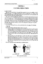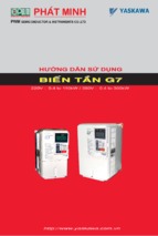design of a standard wheel. Three conditions should be defined for a standard wheel design: Part B 17.2 17.2.1 Types of Wheels 1. the determination of the two offsets d and b 2. a mechanical design that allows steering motion or not (i. e., to fix the wheel orientation or not) 3. the determination of steering and driving actuation (i. e., active or passive drive) In order to achieve robot locomotion, wheeled mobile robots are widely used in many applications. In general, wheeled robots consume less energy and move faster than other locomotion mechanisms (e.g., legged robots or tracked vehicles). From the viewpoint of control, less control effort is required, owing to their simple mechanisms and reduced stability problems. Although it is difficult to overcome rough terrain or uneven ground conditions, wheeled mobile robots are suitable for a large class of target environments in practical applications. When we think of a single-wheel design, there are two candidates: a standard wheel or a special wheel. A standard wheel can be understood as a conventional tire. Special wheels possess unique mechanical structures including rollers or spheres. Figure 17.1 shows the general Condition 1 is the kinematic parameter design problem for a single standard wheel. The parameter d can be either 0 or some positive constant. Parameter b is the lateral offset of the wheel and is usually set to zero. In a special design, a nonzero b may be selected to obtain pure rolling contact between the wheel and ground without causing rotational slip at the contact point. However, this is rarely used and we mainly consider the case of zero lateral offset b. Condition 2 is a design problem for whether the wheel orientation can be changed or not. If the steering axis is fixed, the wheel provides a velocity constraint on the driving direction. Condition 3 is the design problem of whether to actuate steering or driving motion by actuators or to drive steering or motion passively. Wheeled Robots a) 17.2 Mobility of Wheeled Robots 393 a) YR b) β Robot chassis l α A υ p XR b) X1 d b Caster wheel c) X1 B b A d B β d d l β A α Robot chassis p l p A α X2 c) YR Robot chassis X2 β (t) Fig. 17.1a–c The general design of a standard wheel. 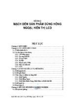(a) side view (b) front view (c) top view l p α A υ XR Fig. 17.2a–c Structures of standard wheels. (a) Passive fixed wheel. (b) Passive or active, off-centered orientable wheel. (c) Active orientable wheel without offsets In such a case, the steering motion should not be passive because the wheel orientation cannot be changed passively. However, the driving velocity can be determined passively by actuation of other wheels. Wheel orientation should be actively steered to the desired velocity direction due to the nonholonomic velocity constraint. This implies that the wheel orientation should be aligned before movement. In summary, four types of standard wheels are commonly used. The first is a passively driven wheel with Part B 17.2 If steering motion is allowed, the offset d plays a significant role in the kinematic modeling. For a conventional caster wheel (i. e., an off-centered orientable wheel), there is a nonzero offset d. Point A in Fig. 17.1 indicates the location of the joint connecting the wheel module to the robot chassis. Two orthogonal linear velocity components at point A are obtained by a caster wheel, which result from the steering and driving motions of the wheel module. This implies that a passive caster wheel does not provide an additional velocity constraint on the robot’s motion. If a caster wheel is equipped with two actuators that drive steering and driving motions independently, holonomic omnidirectional movement can be achieved because any desired velocity at point A can be generated by solving the inverse kinematics problem. If the offset d is set to zero, the allowable velocity direction at point A is limited to the wheel orientation. 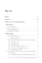Robot chassis 394 Part B Robot Structures Fig. 17.3 (a) Swedish wheel. (b) Attachment of a Swedish wheel and (c) spherical wheel [17.2] a) b) X2 β γ Robot chassis A l α p c) X1 ω0 Drive roller Motor ω1 Y θ= 0 Encoders Part B 17.2 ω2 X a fixed steering axis. The second is a passive caster wheel with offset d. The third is an active caster wheel with offset d, where the steering and driving motions are con- trolled by actuators. The fourth is an active orientable wheel with zero offset d, where steering and driving motions are driven by actuators. The structures of each wheel type are shown in Fig. 17.2. The kinematics and constraints of those wheels will be explained in detail in Sect. 17.2.2. Although standard wheels are advantageous because of their simple structure and good reliability, the nonholonomic velocity constraint (i. e., no side-slip condition) limits robot motion. On the other hand, special wheels can be employed in order to obtain omnidirectional motion of a mobile robot (omnimobile robot), i. e., to ensure three degrees of freedom for plane motion. We consider two typical designs of special wheels: the Swedish wheel and the spherical wheel. Figure 17.3a shows the Swedish wheel. Small passive free rollers are located along the outer rim of the wheel. Free rollers are employed in order to eliminate the nonholonomic velocity constraint. Passive rollers are free to rotate around the axis of rotation, which results in lateral motion of the wheel. As a result, a driving velocity should be controlled, while the lateral velocity is passively determined by the actuation of the other wheels. A spherical wheel is shown in Fig. 17.3c. The rotation of the sphere is constrained by rollers that make rolling contact with the sphere. The rollers can be divided into driving and supporting rollers. The sphere is driven by actuation of the driving rollers, whereas the rolling contacts provide nonholonomic constraints, and the resultant motion of the sphere module becomes holonomic. This implies that the robot can be moved with any desired linear/angular velocities at any time. By using the spherical wheel, a holonomic omnidirectional mobile robot can be developed and the robot achieves smooth and continuous contact between the sphere and the ground. However, the design of the sphere-supporting mechanism is difficult and the payload must be quite low due to the point contact. Another drawback is that the surface of the sphere can be polluted when traveling over dirty ground and it is difficult to overcome irregular ground conditions. These drawbacks limit the practical application of the spherical wheel. An example of the use of spherical wheels can be found in [17.2] and [17.3]. The spherical structure can also be applied to special robotic transmissions; examples include the nonholonomic manipulator in [17.4] and the passive haptic system in [17.5]. Wheeled Robots We assume, as a first step, that the mobile robot under study is made up of a rigid cart equipped with nondeformable wheels, and that it is moving on a horizontal plane. The position of the robot on the plane is described, with respect to an arbitrary inertial frame, by the posture vector ξ = (x y θ)T , where x and y are the coordinates of a reference point P of the robot cart, while θ describes the orientation of a mobile frame attached to the robot, with respect to the inertial frame (Fig. 17.4). We assume that, during motion, the plane of each wheel remains vertical and the wheel rotates around its horizontal axle, whose orientation with respect to the cart can be fixed or varying. We distinguish between two basic classes of idealized wheels, namely conventional and the Swedish wheels. In each case, it is assumed that the contact between the wheel and the ground is reduced to a single point. The kinematic constraints result from the fact that the velocity of the material point of the wheel in contact with the ground is equal to zero. For a conventional wheel, the kinematic constraints imply that the velocity of the center of the wheel is parallel to the wheel plane (nonslip condition) and is proportional to the wheel rotation velocity (pure rolling condition). For each wheel the kinematic constraints therefore result in two independent conditions. For a Swedish wheel, due to the relative rotation of the rollers with respect to the wheel, only one of the velocity components of the wheel contact point is zero. The direction of this zero component is fixed with respect to the wheel plane and depends on the wheel construction. l2 X2 X1 Conventional Wheels We now derive the general form of the kinematic constraints for a conventional wheel. As shown in Fig. 17.2, there are several variations of the conventional wheel design. First, we focus on the off-centered orientable wheel in Fig. 17.2b. The center of the wheel, B, is connected to the cart by a rigid rod from A (a fixed point on the cart) to B, aligned with the wheel plane. The rod, whose length is denoted by d, can rotate around a fixed vertical axle at point A. The position of A is specified by two constant polar coordinates, l and α, with respect to the reference point P. The rotation of the rod with respect to the cart is represented by the angle β. The radius of the wheel is denoted by r, and its angle of rotation around its horizontal axle is denoted ϕ. The description therefore involves four constant parameters: α, l, r, and d, and two variables: ϕ(t) and β(t). With these notations the kinematic constraints are derived as follows. We make the derivation explicit for the general situation corresponding to a caster wheel (Fig. 17.2b). For fixed or steering wheels one just has to consider either the case d = 0 and constant β (fixed wheels), or d = 0 and variable β (steering wheels). First we evaluate the velocity of the center of the wheel, which results from the following vector expresd d d d sion dt OB = dt OP + dt PA + dt AB. The two components of this vector in the robot frame are expressed ˙ ˙ ˙ as: x cos θ + y sin θ − l θ sin α + (θ + β)d cos(α + β) and ˙ ˙ ˙ ˙ ˙ −x sin θ + y cos θ − l θ cos α + (θ + β)d sin(α + β). ˙ ˙ The projections of this vector onto the direction of the wheel plane, i. e., onto the vector (cos(α + β − π/2), sin(α + β − π/2)) and the vector of the wheel axle (cos(α + β), sin(α + β)), are r ϕ and 0, respectively, ˙ corresponding to the pure rolling and nonslip conditions. After some manipulations, these conditions can be rewritten in the following compact form. Pure rolling condition: ˙ (− sin(α + β) cos(α + β) l cos β)R(θ)ξ + r ϕ = 0 , ˙ θ Robot chassis 395 For such wheels the kinematic constraints result in only one condition. 17.2.2 Kinematic Constraints y 17.2 Mobility of Wheeled Robots (17.1) P ˙ ˙ (− cos(α + β) sin(α + β) d + l sin β)R(θ)ξ + d β =0. (17.2) x l1 Fig. 17.4 The posture definition of a mobile robot on a plane In these expressions R(θ) is the orthogonal rotation matrix expressing the orientation of the robot with Part B 17.2 Nonslip condition: 396 Part B Robot Structures respect to the inertial frame, i. e., ⎛ ⎞ cos θ sin θ 0 ⎜ ⎟ R(θ) = ⎝− sin θ cos θ 0⎠ . 0 0 • (17.3) 1 As said before, these general expressions can be simplified for the different types of conventional wheels. For fixed wheels, the center of the wheel is fixed with respect to the cart and the wheel orientation is constant. This corresponds to a constant value of β and d = 0 (Fig. 17.2a). The nonslip equation (17.2) then reduces to ˙ (cos(α + β) sin(α + β) l sin β)R(θ)ξ = 0 . (17.4) For steering wheels, the center of the wheel is also fixed with respect to the cart (i. e., d = 0), with β timevarying, so the nonslip equation takes the form (17.2). This structure was already introduced in Fig. 17.2c. The situation described by (17.1) and (17.2), with a nonzero-length rod AB and time-varying orientation angle β corresponds to caster wheels. Swedish Wheels The position of a Swedish wheel with respect to the cart is described, as for a fixed wheels, by three constant parameters: α, β, and l. An additional parameter is required to characterize the direction, with respect to the wheel plane, of the zero component of the velocity at the contact point of the wheel. This parameter is γ , which is the angle between the axle of the rollers and the wheel plane (Fig. 17.3b). The kinematic constraints now impose only one condition: (− sin(α + β + γ ) cos(α + β + γ ) l cos(β + γ )) ˙ (17.5) × R(θ)ξ + r cos γ ϕ = 0 . ˙ 17.2.3 Robot Configuration Variables Part B 17.2 We now consider a wheeled robot equipped with N wheels of the above described types. We use the following subscripts to identify quantities related to these four types: ‘f’ for fixed wheels, ‘s’ for steering wheels, ‘c’ for caster wheels, and ‘sw’ for Swedish wheels. The numbers of wheels of each type are denoted by Nf , Ns , Nc , and Nsw , with N = Nf + Ns + Nc + Nsw . The configuration of the robot is fully described by the following generalized coordinate vector. • posture coordinates: the posture vector ξ(t) = (x(t) y(t) θ(t)) ; • orientation coordinates: the Ns + Nc orientation angles of the steering and caster wheels, i. e., β(t) = (βs (t) βc (t)) ; rotation coordinates: the N rotation angles of the wheels, i. e., ϕ(t) = (ϕf (t) ϕs (t) ϕc (t) ϕsw (t)) This whole set of coordinates is termed the set of configuration coordinates. The total number of configuration coordinates is Nf + 2Ns + 2Nc + Nsw + 3. 17.2.4 Restriction on Robot Mobility The pure rolling conditions for fixed, steering, and caster wheels, as well as the constraints relative to the Swedish wheels, can be written in the following compact form ˙ J1 (βs , βc )R(θ)ξ + J2 ϕ = 0 , ˙ with (17.6) ⎛ ⎞ J1f ⎜ ⎟ ⎜ J (β ) ⎟ J1 (βs , βc ) = ⎜ 1s s ⎟ . ⎝ J1c (βc )⎠ J1sw In this expression J1f , J1s (βs ), J1c (βc ), and J1sw are, respectively, (Nf × 3), (Ns × 3), (Nc × 3), and (Nsw × 3) matrices, whose forms derive directly from the kinematic constraints, while J2 is a constant (N × N) diagonal matrix whose entries are the radii of the wheels, except for the radii of the Swedish wheels which are multiplied by cos γ . The value γ = π would correspond to the direction 2 of the zero component of the velocity being orthogonal to the plane of the Swedish wheel. Such a wheel would be subject to a constraint identical to the nonslip condition for a conventional wheel, hence losing the benefit of implementing a Swedish wheel. This implies that γ = π 2 and that J2 is a nonsingular matrix. The nonslip conditions for caster wheels can be summarize as ˙ ˙ C1c (βc )R(θ)ξ + C2c βc = 0 , (17.7) where C1c (βc ) is a (Nc × 3) matrix, whose entries derive from the nonslip constraints (17.2), while C2c is a constant diagonal nonsingular matrix, whose entries are equal to d. The last constraints relate to the nonslip conditions for fixed and steering wheels. They can be summarized as ∗ ˙ C1 (βs )R(θ)ξ = 0 , (17.8) Wheeled Robots where C1f ∗ C1 (βs ) = C1s (βs ) 17.2 Mobility of Wheeled Robots a) , where C1f and C1s (βs ) are, respectively, Nf × 3 and Ns × 3 matrices. It is important to point out that the restrictions on robot mobility result only from the conditions (17.8) involving the fixed and the steering wheels. These condi∗ ˙ tions imply that the vector R(θ)ξ belongs to N[C1 (βs )], ∗ (β ). For any R(θ)ξ satis˙ the null space of the matrix C1 s fying this condition, there exists a vector ϕ and a vector ˙ ˙ βc satisfying, respectively, conditions (17.6) and (17.7), because J2 and C2c are nonsingular matrices. ∗ Obviously rank[C1 (βs )] ≤ 3. If it is equal to 3 then ˙ = 0, which means that any motion in the plane is R(θ)ξ impossible. More generally, restrictions on robot mobil∗ ity are related to the rank of C1 (βs ), as will be discussed in detail below. It is worth noticing that condition (17.8) has a direct geometrical interpretation. At each time instant the motion of the robot can be viewed as an instantaneous rotation about the instantaneous center of rotation (ICR), whose position with respect to the cart can be time varying. At each instant the velocity of any point of the cart is orthogonal to the straight line joining this point and the ICR. This is true, in particular, for the centers of the fixed and steering wheels, which are fixed points of the cart. On the other hand, the nonslip condition implies that the velocity of the wheel center is aligned with the wheel plane. These two facts imply that the horizontal rotation axles of the fixed and steering wheels intersect at the ICR (Fig. 17.5). This is equivalent to the condition ∗ that rank[C1 (βs )] ≤ 3. 17.2.5 Characterization of Robot Mobility As said before the mobility of the robot is directly related ∗ to the rank of C1 (βs ), which depends on the design of the robot. We define the degree of mobility δm as ∗ δm = 3 − rank[C1 (βs )] . (17.9) ICR Fig. 17.5a,b The instantaneous center of rotation. (a) A car-like robot; (b) a three-steering-wheels robot ∗ Moreover, we assume that rank[C1 (βs )] = rank(C1f ) + rank[C1s (βs )] ≤ 2. These two assumptions are equivalent to the following set of conditions. 1. If the robot has more than one fixed wheel, they are all on a single common axle. 2. The centers of the steering wheels do not belong to this common axle of the fixed wheels. ∗ 3. The number rank[C1 (βs )] is equal to the number of steering wheels that can be oriented independently in order to steer the robot. We call this number the degree of steerability: δs = rank[C1s (βs )] . (17.10) If a robot is equipped with more than δs steering wheels, the motion of the extra wheels must be coordinated in order to guarantee the existence of the ICR at each instant. We conclude that, for wheeled mobile robot of practical interest, the two defined indices, δm and δs , satisfy the following conditions. 1. The degree of mobility satisfies 1 ≤ δm ≤ 3. The upper bound is obvious, while the lower bound means that we consider only cases where motion is possible. 2. The degree of steerability satisfies 0 ≤ δs ≤ 2. The upper bound can be reached only for robots without fixed wheels, while the lower bound corresponds to robots without steering wheels. 3. The following is satisfied: 2 ≤ δm + δs ≤ 3. The case δm + δm = 1 is not acceptable because it corresponds to the rotation of the robot about a fixed ICR. The cases δm ≥ 2 and δs = 2 are excluded because, according to the above assumptions, δs = 2 implies δs = 1. These conditions imply that only five structures are of practical interest, corresponding to the five pairs (δm , δs ) satisfying the above inequalities, according to Part B 17.2 Let us first examine the case rank(C1f ) = 2, which implies that the robot has at least two fixed wheels. If there are more than two fixed wheels, their axles intersect at the ICR, whose position with respect to the cart is then fixed in such a way that the only possible motion is a rotation of the cart about this fixed ICR. Obviously, from the user’s point of view, such a design is not acceptable. We therefore assume that rank(C1f ) ≤ 1. b) ICR 397 398 Part B Robot Structures the following array. δm 3 2 2 1 1 δs 0 0 1 1 2 Below, each type of structure will be designated by using a denomination of the form type (δm , δs ) robot. 17.2.6 The Five Classes of Wheeled Mobile Robots We now briefly describe the five classes of wheeled robot structures, pointing out the mobility restriction inherent to each class. Details and examples can be found in Sect. 17.5 and in [17.6]. Type (3,0) Robots These robots have no fixed and no steering wheels and are equipped only with Swedish or caster wheels. Such robots are called omnimobile, because they have full mobility in the plane, which means that they are able to move in any direction without any reorientation. Type (2,0) Robots These robots have no steering wheels, but either one or several fixed wheels with a common axle. Mobility is restricted in the sense that, at a given posture ξ(t), the ve˙ locity ξ (t) is constrained to belong to a two-dimensional distribution spanned by the vector fields R (θ)s1 and R (θ)s2 , where s1 and s2 are two constant vectors spanning N(C1f ). A typical example of such a robot is the wheelchair. Type (2,1) Robots These robots have no fixed wheels and at least one steering wheel. If there is more than one steering wheel, their orientations must be coordinated in such ˙ a way that rank[C1s (βs )] = δs = 1. The velocity ξ (t) is constrained to belong to a two-dimensional distribution spanned by the vector fields R (θ)s1 (βs ) and R (θ)s2 (βs ), where s1 (βs ) and s2 (βs ) are two vectors spanning N(C1s (βs )). Type (1,1) Robots These robots have one or several fixed wheels on a single common axle, and also one or several steering wheels, with the conditions that their centers are not located on the common axle of the fixed wheels, and that their orientations are coordi˙ nated. The velocity ξ (t) is constrained to belong to a one-dimensional distribution parameterized by the orientation angle of one arbitrarily chosen steering wheel. Mobile robots built on the model of a conventional car (often called car-like robots) belong to this class. Type (1,2) Robots These robots have no fixed wheels, but at least two steering wheels. If there are more than two steering wheels, then their orientation must be coordinated in order to satisfy the condition rank[C1s (βs )] = δs = 2. The veloc˙ ity ξ (t) is constrained to belong to a one-dimensional distribution parameterized by the orientation angles of two arbitrarily chosen steering wheels. 17.3 State-Space Models of Wheeled Mobile Robots In this section, the mobility analysis discussed in the previous section is reformulated into a state-space form that will be useful for subsequent developments. We introduce four different kinds of state-space representation that are of interest for understanding the behavior of wheeled robots, and for control design purpose. • Part B 17.3 • • The posture kinematic model, which is the simplest state-space model able to give a global description of the robot, from the users viewpoint. The configuration kinematic model allows one to describe the kinematic behavior of the whole robot, including all the configuration variables. The configuration dynamic model is the most general state-space model. It gives a complete description of • the dynamics including the forces provided by the actuators. In particular, it allows to one address the issue of actuator configuration and to define a criterion to check whether the motorization is sufficient to exploit the kinematic mobility fully. The posture dynamic model, which is feedback equivalent to the configuration dynamic model, constitutes a dynamical counterpart to the posture kinematic model. 17.3.1 Posture Kinematic Models We have shown that, whatever the type of robot, the ve˙ locity vector ξ (t) is restricted to belong to a distribution Wheeled Robots Δc defined as ˙ ξ ∈ Δc = span{col[R (θ)Σ(βs )]} , where the columns of the matrix Σ(βs ) constitute a ba∗ sis of N[C1 (βs )]. This is equivalent to the following statement: for all t, there exists a vector η such that ˙ ξ = R (θ)Σ(βs )η , (17.11) The dimension of the distribution Δc , and hence of the vector η(t), is equal to the degree of mobility δm of the robot. Obviously, in the case where the robot has no steering wheels, the matrix Σ is constant, and the expression (17.11) reduces to ˙ ξ = R (θ)Ση . (17.12) In the opposite case (δs ≥ 1), the matrix Σ explicitly depends on the orientation angles βs , and the expression (17.11) can be augmented as follows: ˙ ξ = R (θ)Σ(βs )η , ˙ βs = ς . (17.13) (17.14) 399 the inputs ς(t). However, the action of ς(t) on the pos˙ ture coordinates ξ (t) is indirect, since it is achieved only through the coordinates βs , which are related to the inputs ς(t) by an integral action, reflecting the fact that the modification of the orientation of a steering wheel cannot be achieved instantaneously. The maneuverability of a wheeled robot depends not only on δM , but also on the way these δM degrees of freedom are partitioned into δm and δs . Therefore, two indices are needed to characterize the maneuverability. Obviously the ideal situation is that of omnimobile robots where δM = δm = 3. In order to avoid useless notational complications, we will assume from now on that the degree of steerability is equal to the number of steering wheels, i. e., Ns = δs . This is a restriction from a robot design viewpoint. However, for the mathematical analysis of the behavior of mobile robots, there is no loss of generality in this assumption, although it considerably simplifies the technical derivation. Indeed, for robots with an excess of steering wheels, it is always possible to reduce the condition (17.8) to a minimal subset of exactly δs independent constraints that correspond to the δs wheels that have been selected as the master steering wheels and to ignore the other slave wheels in the analysis. 17.3.2 Configuration Kinematic Models In order to discuss the restriction of mobility, we have considered only a subset of the conditions induced by the kinematic constraints, namely the nonslip conditions for the fixed and steering wheels (17.8). The remaining constraints are now used to derive the equations of evolution of the rotation velocities ϕ and of the orientation ˙ ˙ velocities of the caster wheels βc . From (17.6) and (17.7) it follows immediately that −1 ˙ ˙ βc = −C2c C1c (βc )R(θ)ξ , −1 ˙ ϕ = −J2 J1 (βs , βc )R(θ)ξ . ˙ (17.15) (17.16) By combining these equations with the posture kinematic model (17.13), the state equations for βc and ϕ become ˙ βc = −D(βc )Σ(βs )η , ϕ = −E(βs , βc )Σ(βs )η , ˙ where −1 D(βc ) = −C2c C1c (βc ) and −1 E(βs , βc ) = −J2 J1 (βs , βc ) . (17.17) (17.18) Part B 17.3 The representation (17.12) (or (17.13) and (17.14)) can be viewed as a state-space representation of the model, reflecting the mobility restriction induced by the constraints; it is termed the posture kinematic model. The state vector is constituted by the three posture ˙ coordinates ξ (t) and, possibly, by δs orientation coordinates βs . The vectors η and ξ, of dimension δm and δs , respectively, are homogeneous to velocities and can be interpreted as control inputs entering the model linearly. Nevertheless, this interpretation should be treated with some care, since the true physical inputs are the torques provided by the embarked actuators. The kinematic posture model is in fact only a subsystem of the general dynamic model that will be presented in Sect. 17.3.3. This posture kinematic model allows us to discuss further the maneuverability of wheeled robots. The degree of mobility δm is equal to the number of degrees of freedom that can be directly manipulated from the inputs η(t), without reorientation of the steering wheels. Intuitively, it corresponds to how many degrees of freedom the robot could have instantaneously from its current position, without steering any of its wheels. This number δm is not equal to the overall number of degrees of freedom of the robot that can be manipulated from the inputs η(t) and ς(t), which is equal to the sum δM = δm + δs and which we could call degree of maneuverability. It includes the δs degrees of freedom that are accessible from 17.3 State-Space Models of Wheeled Mobile Robots 400 Part B Robot Structures Defining q as the vector of configuration coordinates, i. e., ⎛ ⎞ ξ ⎜ ⎟ βs ⎟ ⎜ q=⎜ ⎟ , ⎝βc ⎠ ϕ the evolution of the configuration coordinates can be described by the following compact form, called the configuration kinematic model q = S(q)u , ˙ where (17.19) ⎛ R (θ)Σ(βs ) ⎜ 0 ⎜ S(q) = ⎜ ⎝ D(βc )Σ(βs ) E(βs , βc )Σ(βs ) and u = η ς ⎞ 0 ⎟ I⎟ ⎟, 0⎠ 0 . (17.20) The vector q is the vector of generalized coordinates allowing one to fully describe the position and the configuration of the mobile robot. The constraints (17.6), (17.7), and (17.8) can be summarized under the following compact form J(q)q = 0 , ˙ (17.21) where the matrix J(q) is the Jacobian of the constraints, i. e., ⎞ ⎛ J1 (βs , βc )R(θ) 0 0 J2 ⎟ ⎜ (17.22) J(q) = ⎝ C1c (βc )R(θ) 0 C2c 0 ⎠ . ∗ C1 (βs )R(θ) 0 0 0 caster wheels, or the orientation of all the wheels. The torques provided by the actuators are denoted τϕ for the rotation of the wheels, τc for the orientation of the caster wheels, and τs for the orientation of the steering wheels. Using the Lagrange formalism, we obtain the following compact equations: d dt ∂T ∂q ˙ − ∂T = τ + J (q)λ . ∂q In this equation 1. T (q, q) the kinetic energy of the robot can be ex˙ pressed as a quadratic form T (q, q) = 1 q T M(βc )q, ˙ ˙ 2˙ where M(βc ) is a symmetric positive-definite matrix. 2. τ is the vector of the generalized forces associated with the torques provided by the actuators ⎛ ⎞ 0 ⎜ ⎟ ⎜ τs ⎟ τ=⎜ ⎟ , ⎝ τc ⎠ τϕ 3. the term J (q)λ is the vector of generalized forces associated with the kinematic constraints. The vector λ is the vector of the Lagrange multipliers associated with the constraints. With the above expression for the kinetic energy (17.19) can be rewritten as M(βc )q + f (q, q) = τ + J (q)λ . ¨ ˙ (17.23) [S (q)M(βc )S(q)]u ˙ ˙ +[S (q)M(βc ) S(q)u + S (q) f (q, S(q)u)] = S (q)τ 17.3.3 Configuration Dynamic Models Part B 17.3 We now derive the dynamic configuration model which constitutes, from a mechanical viewpoint, the full system description, allowing one to relate the control inputs provided by the embarked actuators to the evolution of the generalized coordinates q. This model is derived using the Lagrange formalism. We assume that the robot is equipped with actuators that can force either the orientation of the steering and (17.25) (See Sect. 2.3 on the dynamics of rigid-body systems.) The Lagrange multipliers are eliminated by left multiplying (17.25) by S(q) and using (17.23). Moreover, q ˙ and q can be eliminated using (17.19). ¨ It follows that The two matrices S(q) and J(q) satisfy the relation S(q)J(q) = 0 . (17.24) (17.26) or, more compactly H(q)u + F(q, u) = S (q)τ . ˙ (17.27) This equation, together with the equation of the configuration kinematic model (17.19) constitutes the configuration dynamic model of the robot. In this general formulation (17.27) τ represents all the torques that can potentially be applied for the orientation and rotation of the wheels. In practice, however, only Wheeled Robots a limited number of actuators are used, which means that many components of this vector are identically zero. Our purpose now is to characterize the actuator configurations exploiting the maneuverability that can be expected from the posture kinematic model. First, it is clear that all the steering wheels must be provided with an actuator for their orientation, otherwise these wheels would just play the role of fixed wheels. Moreover, in order to ensure full robot mobility, Nm additional actuators (with Nm ≥ δm ) must be implemented for either the rotation of some wheels or the orientation of some caster wheels. The vector of the torques developed by these additional actuators is denoted by τm , and we can write τc = Pτm , τϕ (17.28) where P is an ((Nc + N) × Nm ) elementary matrix that selects the components of τc and ϕc that appear explicitly in τm and may therefore be used as control inputs. With this notation, the dynamic equation (17.27) can be rewritten as τ = Γ (βs , βc ) s τm , (17.29) where B(βs , βc ) = Σ (βc )(D (βc ) E (βs , βc )) It must be pointed out that the evolution of the variable u can be assigned provided P (and equivalently the actuator implementation) is such that the matrix B(βs , βc )P has full rank for all (βs , βc ). We assume in the sequel that this condition is satisfied, ensuring therefore full exploitation of the potential maneuverability of the robot. 401 This state feedback is given by τs = Γ + (βs , βc ) [H(q)v − F(q, u)] , τm (17.32) where Γ + denotes an arbitrary left inverse of Γ . (See Sect. 6.6 on computer torque control.) We emphasize that a further simplification is of interest from an operational viewpoint. In the context of trajectory planning or feedback control design, it is clear that the user is essentially concerned with controlling the posture of the robot (namely the posture coordinate ξ(t)) by using the control input v. This implies that we can deliberately ignore the coordinates βc and ϕ and restrict our attention to the following posture dynamic model: z = B(z)u , ˙ u=v, ˙ (17.33) (17.34) where z= B(z) = τs τm I 0 H(q)u + F(q, u) = ˙ 0 B(βs , βc )P 17.3 State-Space Models of Wheeled Mobile Robots ξ βs , u= η ς R (θ)Σ(βs ) 0 0 I and . The first equation is nothing but the kinematic posture model equation (17.12), or (17.13,17.14). The difference with this kinematic model is the presence of integrators on the input variables (17.34), so that the variables u are now part of the state vector. This leads to the appearance of a drift term in the dynamic model. The posture dynamic model fully describes the system dynamics between the control input v and the posture ξ. The coordinates βc and ϕ have apparently disappeared but it is important to note that they are in fact hidden in the feedback (17.32). 17.3.5 Articulated Robots 17.3.4 Posture Dynamic Models q = S(q)u , ˙ u=v, ˙ (17.30) (17.31) where v represents a set of (δs + δm ) auxiliary independent control inputs. Up to now we have considered only simple mobile robots, i. e., robots made up of only one cart. In this section we extend this analysis to articulated robots, i. e., robots formed by a master cart with several trailers. A typical example is the well-known truck and trailers system. Each of the trailers can be equipped of wheels of the types described in Sect. 17.2.2, actuated or not. The number of possible structures becomes almost infinite. This is why we restrict our analysis to passive trailers (no onboard actuators) equipped only with fixed wheels. Part B 17.3 It follows from the above assumption that the configuration dynamic model is feedback equivalent (by smooth static time-invariant state feedback) to the following system: 402 Part B Robot Structures We consider a master cart that can be described by any of the five discussed types. The first trailer is connected to the cart, i. e., a material point of the trailer is fixed to a material point of the master cart. The relative position of the trailer with respect to the cart is described by a posture angle θ1 . This trailer is equipped with one or several fixed wheels. If there is more than one wheel, then they have the same geometric axle. To this first trailer is connected a second trailer, of the same type, whose relative position with respect to the first is characterized by the angle θ2 , and so on, for a sequence of Nt trailers. The posture vector allowing one to describe this augmented system is now extended to a 3 + Nt generalized ξ posture vector: ξ ∗ = ∗ , where ξ is the posture vecθ tor of the master cart while θ ∗ is the vector of the relative angles of the successive trailers. We also denote by ξi∗ the posture of a partial system, from the master cart up to the i-th trailer, i. e., ξi∗ = ξ θ1 . . . θi . • • • The reference point is the connection point between trailer (i − 1) and trailer i. We define the posture of trailer i, ξi , by the vector made up by the coordinates of this reference point and the absolute orientation of the trailer, which is equal to (θ + θ1 + . . . + θi ). The position of the wheel with respect to this reference point is described by its polar coordinates αij and lij . The orientation of the wheel is given by the constant angle βij . The rotation angle of the wheel is denoted by ϕij . The pure rolling condition is then given by (− sin(αij + βij ) cos(αij + βij ) lij cos βij ˙ R(θ + θ1 + . . . + θi )ξi + r ϕij = 0 , ˙ (17.35) while the nonslip condition becomes Part B 17.3 cos(αij + βij ) sin(αij + βij ) lij sin βij ˙ R(θ + θ1 + . . . + θi )ξi = 0 . (17.36) The posture vector of trailer i, ξi , can be expressed as a function of ξ and of the orientation angles of the preceding trailers, i. e., ∗ ξi = gi (ξi−1 ) . ˙ ξi = ∂gi ˙ ξ+ ∂ξ i−1 k=1 ∂gi ˙ θk ∂θk ∗ ˙∗ = G i (ξi−1 )ξi−1 i = 1, . . . , Nt . (17.37) Using this expression in the nonslip condition (17.36) for the Nt trailers, and using the nonslip condition for the master cart, we obtain the following set of equations reflecting the restriction of motion for all parts of the system: ˙ J ∗ (βs , θ, θ1 , . . . , θ Nt )ξ ∗ = 0 . (17.38) Following the same lines as in Sect. 17.3.1, we derive the posture kinematic model of the articulated robot: ˙ ξ ∗ = S∗ (βs , θ, θ1 , . . . , θ Nt )η , ˙ βs = ς . (17.39) (17.40) The matrices J ∗ and S∗ satisfy the relation The kinematic constraints relative to the fixed wheel j of trailer i (1 ≤ i ≤ Nt ) can be expressed as in Sect. 17.2.2 using the following notations: • This implies that J ∗ (βs , θ, θ1 , . . . , θ Nt )S∗ (βs , θ, θ1 , . . . , θ Nt ) = 0 . (17.41) Equation (17.37) provides the evolution of the relative angles of each trailer. It must be noticed that the time derivative of each of this angles depends on the input variables relative to the master cart (i. e., η and ς), on βs , if the master cart is equipped with steering wheels, and on the relative angles of the preceding trailers only. This last property is due to the recursive structure of J ∗ and S∗ . Obviously it is possible to derive the three other models of the articulated robot, in a similar way as for the simple robot, as explained in Sects. 17.3.2, 17.3.3, and 17.3.4. For the configuration kinematic model we consider the generalized vector constituted from all the variables, including the rotation angles of the wheels of the trailers. This model is derived as an extension of the posture model taking into account the pure rolling constraints (17.35). It has the form (17.19), with an appropriate definition of q. The configuration dynamic model is derived from the Lagrange equations of the system. It has the form (17.27), while the posture dynamic model, obtained via static state feedback, is again related to the posture kinematic, as for the simple robot (17.33) and (17.34). Wheeled Robots 17.4 Structural Properties of Wheeled Robots Models 403 17.4 Structural Properties of Wheeled Robots Models Our purpose in this section is to discuss the structural properties of the above models of wheeled robots from a control design viewpoint. Since, in most situations, the user is only interested in the posture of the robot, and not in the internal variables (such as the wheel orientation angles), the most interesting models are the posture models (kinematic or dynamic). This is why the discussion on structural properties will be mainly based on the posture models. 17.4.1 Irreducibility, Controllability, and Nonholonomy 1. We first address the question of the reducibility of the kinematic posture state-space model (17.33). A state model is reducible if there exists a change of coordinates such that some of the new coordinates are identically zero along the motion system. For a nonlinear dynamical system without drift like (17.13, 14) reducibility is related to the dimension of ¯ the involutive closure Δ of the following distribution Δ, expressed in local coordinates as Δ(z) = span [colB(z)] . ¯ dim Δ(s) − dim [Δ(s)] = (3 + δs ) − (δm + δs ) = 3 − δm , is related to the nonholonomy of the posture kinematic model. If this difference is nonzero (i. e., if δm ≤ 2) the posture kinematic model is said to be nonholonomic. If δm = 3, which is the case only for omnimobile robots, the kinematic posture model is holonomic. 2. The configuration kinematic model (17.23) is obtained from the posture model by adding the evolution of the internal variables βc (t) and ϕ(t), and takes the same form q = S(q)u. ˙ In order to analyze reducibility and controllability issues we now have to consider the following two distributions: Δ1 (q) = span [col(S(q))], and its in¯ volutive closure Δ1 (q). It follows immediately that ¯ δm + Ns = dim [Δ1 (q)] ≤ dim Δ1 (q) ≤ dim(q) = 3 + N + Nc + Ns . We define the degree of nonholonomy of the configuration kinematic model as ¯ M = dim Δ1 (q) − (δm + δs ) . This number represents the number of velocity constraints that are not integrable and therefore cannot be eliminated from the configuration evolution description, whatever the choice of the generalized coordinates. It must be pointed out that this number depends on the particular structure of the robot, and thus it has not necessarily the same value for two robots belonging to the same class. On the other hand, for a particular choice of generalized coordinates, the number of coordinates that can be eliminated by integration of the constraints is equal to the difference between dim(q) and dim(Δ1 (q)). It can be checked that the configuration kinematic model of all types of wheeled robots (including omnimobile robots) is nonholonomic (i. e., the degree of nonholonomy is not equal to zero), but is reducible. Part B 17.4 A well-known consequence of the Frobenius theorem is that the system is reducible only if ¯ dim(Δ) ≤ dim(Δ) − 1. The following property can be checked for the posture kinematic models of wheeled robots. For the posture kinematic model (17.33) z = B(z)u, ˙ – the input matrix B(z) has full rank, i. e., rank [B(z)] = δm + δs ∀z, ¯ – the involutive distribution Δ(z) has constant ¯ maximal dimension, i. e., dim Δ(z) = 3 + δs . As a consequence, the posture kinematic model of a wheeled robot is irreducible. This is a coordinatefree property. This property has another consequence related to the controllability of the posture kinematic model. For a nonlinear dynamical model without drift of the form (17.13, 14), the strong accessibility algebra co¯ incides with the involutive distribution Δ(z), which has constant maximal dimension. It follows that the strong accessibility rank condition is satisfied and, therefore, the system is strongly accessible from any configuration. For such a driftless system this implies controllability. Practically, this means that a mobile robot can always be driven from any initial posture ξ0 to any final one ξf , in a finite time, by ma. nipulating the velocity control inputs u = η ς Finally, the difference between the dimensions of the ¯ two distributions Δ(z) and Δ(z), i. e., 404 Part B Robot Structures Moreover, it does not satisfy the strong accessibility rank condition. This property does not contradict the irreducibility of the posture kinematic model. The reducibility of the configuration model means that there exists at least one smooth function of q(t), involving explicitly at least one of the variables βc (t) and ϕ(t), that is constant along the trajectories of the system compatible with the full set of kinematic constraints (17.21). 3. We have seen in Sects. 17.3.3 and 17.3.4 that the dynamic models ((17.30, 31), for the configuration model, or (17.33, 34) for the posture model) are related to the corresponding kinematic models, with the difference that the variables are part of the state vector. This implies the existence of a drift term and the fact that the input vector fields are constant. The dynamic models inherit the structural properties of the corresponding dynamic model. In particular, the posture dynamic model is irreducible and small-time locally controllable. 17.4.2 Stabilizability ¯ ¯ Obviously, any arbitrary configuration ξ βs may constitute an equilibrium point for the posture kinematic model. Equilibrium means that the robot is at rest ¯ somewhere, with a given constant posture ξ and a given ¯ constant orientation βs of the steering wheels, and zero velocities, i. e., u = 0. ¯ Let us now consider the question of the existence of a feedback control u(z) able to stabilize a mobile robot at a particular z. ¯ For holonomic robots (i. e., omnimobile robots, for ˙ which z reduces to ξ) the question is trivial, because ξ can be assigned arbitrarily from the input u. For instance the state-feedback control u(z) = B−1 (z)A(z − z), ensures ¯ the following closed-loop dynamics ˙ ¯ ξ = A(ξ − ξ ) , Part B 17.4 and therefore, for any arbitrary Hurwitz matrix A, the exponential stability of the equilibrium z . ¯ For restricted mobility robots (nonholonomic robots) the situation is less favorable. Indeed the so-called Brockett necessary condition for the existence of smooth time-invariant stabilizing feedback is not satisfied, since the map (z, u) → B(z)u is not onto on a neighborhood of the equilibrium z (Sect. 34.4.4). ¯ We conclude that for restricted mobility robots the (nonholonomic) posture kinematic model is not stabilizable by a continuous static time-invariant state feedback. Nevertheless such a model can be stabilized using smooth time-varying state feedback or noncontinuous feedback. This property is inherited by the corresponding dynamic configuration model, which is also not stabilizable by continuous static time-invariant state feedback. 17.4.3 Static State-Feedback Linearizability In this section we analyze the existence of state feedback achieving full or partial linearization of the posture models given by (17.33) for the kinematic model, or (17.33, 34) for the dynamic model. A first result is the following. The largest subsystem of the posture kinematic model (17.33) linearizable by a smooth static feedback has dimension (δm + δs ). The largest linearizable subsystem of the dynamic model (17.33, 34) has dimension 2(δm + δs ). It can be checked that the largest linearizable subsystem of the kinematic posture model is obtained by selecting (δm + δs ) adequate linearizing output functions depending on z. A vector of (3 − δm ) components remains nonlinearized. Similarly the largest linearizable subsystem of the posture dynamic model has dimension 2(δm + δs ), with exactly the same linearizing output functions. For omnimobile robots (i. e., robots with holonomic posture models), δm = 3 and δs = 0. The above property implies that the posture models are fully linearizable by static state feedback. In contrast, restricted mobility robots posture models are only partially linearizable. 17.4.4 Dynamic State-Feedback Linearizability – Differential Flatness The purpose of this section is to show that posture models of wheeled robots can be fully linearized by dynamic state feedback. Obviously we only consider restricted mobility robots, because omnidirectional robots are fully linearizable by static state feedback, as discussed in the previous section. Consider a nonlinear dynamical system given in general state-space form, affine in the inputs m gi (z)ui , z = f (z) + ˙ (17.42) i=1 where the state z ∈ Rn , the input u ∈ Rm , and the vector fields f and gi are smooth. When the system is not completely linearizable by diffeomorphism and static state feedback (as for Wheeled Robots restricted mobility robots), full linearization can nevertheless possibly be achieved by considering more general dynamic feedback laws of the form u = α(z, χ, w) , χ = a(z, χ, w) , ˙ (17.43) where w is an auxiliary control input. Such a dynamic feedback is obtained through the choice of m suitable linearizing output functions yi = h i (z) , i = 1, . . . , m . (17.44) We apply the so-called dynamic extension algorithm to system (17.42)–(17.44). The idea of this algorithm is to delay some combinations of inputs simultaneously affecting several outputs, via the addition of integrators, in order to enable other inputs to act in the meanwhile and therefore hopefully to extend an extended decoupled system of the form (r ) yk k = wk , k = 1, . . . , m , (17.45) (i) where yk denotes the i-th derivative of yk with respect to time, rk is the relative degree of yk , and wk denote the new auxiliary inputs. In order to get a full linearization, we shall have for the n e -dimensional extended system m ri = n e , (17.46) i=1 17.5 Wheeled Robot Structures 405 where n e is the dimension of the extended state vector ze = z χ . If the condition (17.46) is satisfied, then (r −1) ς = Ψ (z e ) = (y1 . . . y1 1 (r . . . ym . . . ymm −1) ) is a local diffeomorphism. A system that can be shown to be linearizable by using the dynamic extension algorithm is an example of a so-called differentially flat system. The linearizing outputs yi = h i (z) are also called flat outputs. Conversely, differential flatness refers by definition to a system that can be linearized by dynamic state feedback. Roughly speaking, for a flat system, the state and the inputs can be expressed as algebraic functions of the flat outputs and their successive time derivatives. These two related properties of linearizability by dynamic state feedback and differential flatness will be of interest for control design and path planning problems. The fact that the posture kinematic and dynamic models of restricted mobility robots are differentially flat systems result directly from the following two properties. 1. Any controllable driftless system with m inputs and at most m + 2 states is a differentially flat system. 2. If a nonlinear system z = f (z, u) is differentially flat, ˙ then the augmented system z = f (z, u), u = v is also ˙ ˙ a differentially flat system and is therefore generically fully linearizable by dynamic state feedback. 17.5 Wheeled Robot Structures There are many design alternatives for wheeled mobile robots. Design problems of a single-body mobile robot include the selection of wheel types, the placement of wheels, and the determination of the kinematic parameters. Design objectives should be specified according to the target environments and tasks, as well as the initial and operational costs of a robot. In this section, robot structures are classified according to the number of wheels, and then features will be introduced focusing on commonly adopted designs. A robot with a single wheel is basically unstable without dynamic control in order to maintain its balance of a body. A typical example is a unicycle. 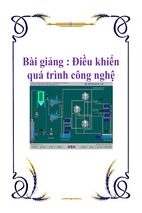As a variation of a unicycle, a robot with a rugby-ball-shaped wheel 17.5.2 Robots with Two Wheels In general, there are two types of two-wheel robots, as shown in Fig. 17.6. Figure 17.6a shows a bicycle- Part B 17.5 17.5.1 Robots with One Wheel can be used in order to improve stability in the lateral direction, as studied in [17.7]. A spherical robot can also be considered as a singlewheel robot. A balancing mechanism such as a spinning wheel is employed to achieve dynamic stability. This approach has advantages including high maneuverability and low rolling resistance. However, single-wheel robots are rarely used in practical applications, because additional balancing mechanisms are required, control is difficult, and pose estimation by pure dead reckoning is not available. An example of a spherical robot can be found in [17.8]. 406 Part B Robot Structures a) Robot chassis Active fixed wheel Passive, actively steerable wheel b) Active fixed wheel Robot chassis Active fixed wheel Fig. 17.6 (a) Bicycle-type robot, (b) inverted-pendulum- type robot Part B 17.5 type robot. It is common to steer a front wheel and to drive a rear wheel. Since the dynamic stability of a bicycle-type robot increases with its speed, a balancing mechanism is not necessarily required. The advantage of this approach is that the robot width can be reduced. However, a bicycle type is rarely used because it cannot maintain its pose when the robot stands still. Fig. 17.6b shows an inverted-pendulum-type robot. It is a two-wheel differential drive robot. It is possible to achieve static stability by accurately placing the center of gravity on the wheel axle. However, it is common to apply dynamic balancing control, which is similar to the conventional control problem for an inverted pendulum. The size of a robot can be reduced by using two-wheel robots, when compared with robots with more than three wheels. A typical application of a pendulum-type robot is to design a structure as a four-wheel robot, consisting of two pendulum robots connected. Then, the robot can climb stairs by lifting its front wheels while the robot reaches the stair. A major disadvantage is that control effort is always required for dynamic balancing. Examples of inverted-pendulum-type robots can be found in [17.9] and [17.10]. 17.5.3 Robots with Three Wheels Since a robot with three wheels is statically stable and has a simple structure, it is one of the most widely used structures for wheeled robots. There are a large number of designs according to the choice of individual wheel types. Every wheel introduced in Sect. 17.2.1 can be used to construct three-wheel robots. In this section, five popular design examples are described: (1) two-wheel differential drive, (2) synchronous drive, (3) an omnimobile robot with Swedish wheels, (4) an omnimobile robot with active caster wheels, and (5) an omnidirectional robot with steerable wheels. Two-Wheel Differential-Drive Robot A two-wheel differential-drive robot is one of the most popular designs and is composed of two active fixed wheels and one passive caster wheel. The robot can be classified as a type (2,0) robot in the nomenclature of Sect. 17.2.6. It is possible to extend the robot to a fourwheel robot by adding passive caster wheels. The major advantages of the robot can be summarized as follows: • • • A simple mechanical structure, a simple kinematic model, and low fabrication cost. A zero turning radius is available. For a cylindrical robot, the obstacle-free space can easily be computed by expanding obstacle boundaries by the robot radius r. Systematic errors are easy to calibrate. On the other hand, its drawbacks are: • • difficulty of moving irregular surfaces. When the robot goes over uneven surfaces, its orientation might change abruptly if one of the active wheels loses contact with the ground; only bidirectional movement is available. Synchronous-Drive Robot A synchronous-drive robot can be built by using centered or off-centered orientable wheels. The steering and driving motions of each wheel are mechanically coupled by chains or belts, and the motions are actuated synchronously, so the wheel orientations are always identical. The kinematic model of a synchronous drive robot is equivalent to that of the unicycle, a type (1,1) robot. Therefore, omnidirectional motion, i. e., motion in any direction, can be achieved by steering the wheel orientations to the desired velocity direction. However, the orientation of the robot chassis cannot be changed. Sometimes a turret is employed to change the body orientation. The most significant advantage of the synchronous-drive robot is that omnidirectional movement can be achieved by using only two actuators. Since the mechanical structure guarantees synchronous steer- Wheeled Robots a) Passive caster wheel b) 17.5 Wheeled Robot Structures 407 x2 Steering pulley Drive pulley v (t ) Wheel ω (t ) v (t ) v (t ) (x,y) ω (t ) Steering motor x1 Steering belt Drive belt ω (t ) Y Drive motor X Y X Active fixed wheel c) d) e) Steering wheels L P L X2 L P Caster wheel X1 X2 P X2 Caster wheel X1 X1 Fig. 17.7 (a) Two-wheel differential drive, (b) synchronous drive, (c) omnimobile robot with Swedish wheels, (d) omnimobile robot with active caster wheels, (e) omnidirectional robot with active steerable wheels ing and driving motions, less control effort is required for motion control. Other advantages include that odometry information is relatively accurate and driving forces are evenly distributed among all the wheels. The drawbacks of this approach can be summarized as • • • complicated mechanical structure if backlash or loose coupling is present in the chain transmission, velocity differences between wheels may occur in order to achieve omnidirectional movement, the wheel orientations should be aligned to the desired velocity direction before movement, due to the nonholonomic velocity constraints. Omnimobile Robot with Active Caster Wheels A holonomic omnidirectional robot can be constructed by using at least two active caster wheels, and the robot Part B 17.5 Omnimobile Robot with Swedish Wheels The omnimobile robot with Swedish wheels corresponds to type (3,0) in the nomenclature of Sect. 17.2.6. At least three Swedish wheels are required to build a holonomic omnidirectional robot. A major advan- tage of using the Swedish wheel is that omnidirectional mobile robots can be easily constructed. At least three Swedish wheels are required to build a holonomic omnidirectional robot. Since omnidirectional robots can be built without using active steering of wheel modules, the mechanical structures of actuating parts can have simple structures. However, the mechanical design of a wheel becomes slightly complicated. One drawback of the Swedish wheel is that there is a vertical vibration because of discontinuous contacts during motion. In order to solve this problem, a variety of mechanical designs have been proposed; examples can be found in [17.11] and [17.12]. Another drawback is its relatively low durability when compared to conventional tires. An example of a robot using Swedish wheels can be found in [17.13]. 408 Part B Robot Structures also belongs to type (3,0). The robot can be controlled to generate arbitrary linear and angular velocities regardless of the wheel orientations. Since the robot uses conventional tires, the disadvantages of Swedish wheels, for example, vertical vibrations or durability problems, can be solved. An example can be found in [17.14]. The disadvantages of this robot can be summarized as follows: • • • • Since the location of the ground contact point (i. e., footprint) changes with respect to the robot chassis, instability can take place when the distance between the wheels is too short. If the robot switches its movement to the reverse direction, an abrupt change of wheel orientations may take place. This is called the shopping-cart effect, which may result in instantaneous high steering velocities. If a driving motor is directly attached to the wheel, wires to the motor will be wound due to steering motions. In order to avoid this, a gear train should be employed to transmit the input angular velocity from the driving motor, which is attached to the robot chassis. In this case, the mechanical structure becomes quite complicated. If a robot is equipped with more than two active caster wheel modules, more than four actuators are used. Since the minimum number of actuator to achieve holonomic omnidirectional motion is three, this is an overactuated system. Therefore, actuators should be accurately controlled in a synchronous way. Part B 17.5 Omnidirectional Robot with Steerable Wheels Centered orientable wheels are also employed to build omnidirectional robots; at least two modules are required. A significant difference between the active caster wheel and the centered orientable wheel is that the wheel orientation should always be aligned with the desired direction of velocity direction, as computed by inverse kinematics. This fact implies that this robot is nonholonomic and omnidirectional: it is a type (1,2) robot. The control problem is addressed in [17.15]. The mechanical drawbacks are similar to those of using active caster wheels (i. e., many actuators and complicated mechanical structures). Since the driving motor is directly attached to the driving axis in many cases, allowable steering angles are limited in order to prevent wiring problems. There are a lot of design candidates for three-wheel robots, other than the five designs described above. They can be classified and analyzed according to the scheme presented in Sect. 17.1. The above designs can be extended to four-wheel robots to improve stability. Additional wheels can be passive wheels without adding additional kinematic constraints. Active wheels can also be added and should be controlled by solving the inverse kinematics problem. Four-wheeled robots require suspension to maintain contact with the ground to prevent wheels from floating on irregular surfaces. 17.5.4 Four Robots with Four Wheels Among the various four-wheel robots, we focus on the car-like structure. The front two wheels should be synchronously steered to keep the same instantaneous center of rotation. Therefore, this solution is kinematically equivalent to a single orientable wheel and the robot can be classified as a type (1,1) robot. A major advantage of a car-like robot is that it is stable during high-speed motion. However, it requires a slightly complicated steering mechanism. If the rear wheels are actuated, a differential gear is required to obtain pure rolling of the rear wheels during the turning motion. If the steering angle of the front wheel cannot reach 90◦ , the turning radius becomes nonzero. Therefore, parking motion control in a cluttered environment becomes difficult. 17.5.5 Special Applications of Wheeled Robots Articulated Robots As explained in Sect. 17.3.5, a robot can be extended to an articulated robot, which is composed of a robot and trailers. A typical example is the luggage-transporting trailer system at airports. By exploiting trailers, a mobile robot obtains various practical advantages. For example, modular and reconfigurable robots can change their configuration according to service tasks. A common design is the car with multiple passive trailers that was presented in Sect. 17.3.5, which is the simplest design of an articulated robot. From the viewpoint of control, some significant issues have been made clear, including a proof of controllability and the development of open- and closed-loop controllers using canonical forms such as the chained form. The design issues for trailer systems are the selection of wheel types and decisions regarding the link parameters. In practical applications, it is advantageous if trailers can move along the path of the towing robot. Passive trailers can follow the path of a towing robot within a small error by using a special Wheeled Robots design of passive steering mechanism for trailers; see, for example, [17.16]. On the other hand, active trailers can be used. There are two types of active trailers. A first approach is to actuate wheels of trailers. The connecting joints are passive, and two-wheel differential-drive robots can be used as active trailers. By using this type of active trailers, accurate path-following control can be achieved. The second approach is to actuate connecting joints. The wheels of the trailer are passively driven. By appropriate actuation of the connecting joints, the robot can move without wheel actuation, by snake-like motions. As an alternative design, we can use an active prismatic joint to connect trailers, in order to lift the neighboring trailer. By allowing vertical motion, a trailer system can climb stairs and traverse rough terrain. Examples of active trailers can be found in [17.17]. Hybrid Robots A fundamental difficulty of using wheels is that they can only be used on flat surfaces. To overcome this problem, wheels are often attached to a special link mechanism. Each wheel is equipped with independent actuators and a linkage mechanism enables the robot to adapt its configuration to irregular ground conditions. A typical design can be found in [17.18] and can be understood as a hybrid robot that is a combination of a legged robot and a wheeled robot. Another hybrid example is a robot equipped with both tracks and wheels. Wheels and tracks have complementary advantages and disadvantages. Wheeled robots are energy efficient, however, tracked robots can traverse rough terrain. Therefore, 17.6 Conclusions 409 θ z s Fig. 17.8 An active trailer system [17.17] 1 2 3 4 Fig. 17.9 A mobile robot for rough terrain [17.18] a hybrid robot can selectively choose its driving mechanism according to environmental conditions, although fabrication cost increases. 17.6 Conclusions that pure rolling and nonslip conditions are satisfied for each wheel. These conditions lead to the kinematic constraints that constitute the basis of the analysis, and particularly of the properties related to the nonholonomy of these models. All model-based control designs therefore also rely on the same assumptions. These assumption are an idealization of the physical reality: these kinematic constraints are not satisfied exactly, and the contact effects are characterized by local slipping effects that are related through phenomenological laws to the contact forces. A question then arises immediately: what is the level of confidence in these models? Using a singular perturbation approach it has been shown that sliding effects can be considered as fast dynamics, with charac- Part B 17.6 The number of possible wheeled mobile robots realizations is almost infinite, depending on the number, type, implementation, geometric characteristics, and motorization of the wheels. This chapter describes several such realizations. Notwithstanding this variety it is possible to classify WMRs into only five generic categories. The (kinematic and dynamic) posture models have exactly the same structure within each of these classes. This fact is crucial for a model-based control design approach, such as that presented in Chap. 34. The discussion of mobility and the derivation of the models are based on assumptions concerning the contact between the ground and the wheels: it is assumed 410 Part B Robot Structures teristic times that are short compared to the dynamics of the global motion of the WMR and can be neglected, at least for analysis and control design purposes (see, for instance, [17.1]). References 17.1 17.2 17.3 17.4 17.5 17.6 17.7 17.8 17.9 B. dAndrea-Novel, G. Campion, G. Bastin: Control of wheeled mobile robots not satisfying ideal velocity constraints: a singular perturbation approach, Int. J. Robust Nonlin. Control 5, 243–267 (1995) H. Asama, M. Sato, L. Bogoni: Development of an omnidirectional mobile robot with 3 DOF decoupling drive mechanism, Proc. IEEE International conference on robotics and automation (1995) pp. 1925–1930 L. Ferriere, G. Campion, B. Raucent: ROLLMOBS, a new drive system for omnimobile robots, Robotica 19, 1–9 (2001) W. Chung: Nonholonomic Manipulators. In: Springer Tracts Adv Robot, Vol. 13 (Springer, Heidelberg 2004) J.E. Colgate, M. Peshkin, W. Wannasuphoprasit: Nonholonomic haptic display, Proc. 1996 IEEE International Conference on Robotics and Automation (1996) pp. 539–544 G. Campion, G. Bastin, B. dAndrea-Novel: Structural properties and classification of kinematic and dynamic models of wheeled mobile robots, IEEE Trans. Robot. Autom. 12, 47–62 (1996) R. Nakajima, T. Tsubouchi, S. Yuta, E. Koyanagi: A development of a new mechanism of an autonomous unicycle, Proc. 1997 IEEE/RSJ International Conference on Intelligent Robots and Systems (1997) pp. 906–912 G.C. Nandy, X. Yangsheng: Dynamic model of a gyroscopic wheel, Proc. 1998 IEEE International Conference on Robotics and Automation (1998) pp. 2683–2688 Y. Ha, S. Yuta: Trajectory tracking control for navigation of self-contained mobile inverse pendulum, Proc. IEEE/RSJ International Conference on 17.10 17.11 17.12 17.13 17.14 17.15 17.16 17.17 17.18 Intelligent Robots and Systems (1994) pp. 1875– 1882 Y. Takahashi, T. Takagaki, J. Kishi, Y. Ishii: Back and forward moving scheme of front wheel raising for inverse pendulum control wheel chair robot, Proc. IEEE International Conference on Robotics and Automation (2001) pp. 3189–3194 K.-S. Byun, S.-J. Kim, J.-B. Song: Design of continuous alternate wheels for omnidirectional mobile robots, Proc. IEEE International conference on robotics and automation (2001) pp. 767–772 M. West, H. Asada: Design and control of ball wheel omnidirectional vehicles, Proc. IEEE International conference on robotics and automation (1995) pp. 1931–1938 B. Carlisle: An omnidirectional mobile robot. In: Development in Robotics (IFS Publ. Ltd., Bedford 1983) pp. 79–87 M. Wada, S. Mori: Holonomic and Omnidirectional Vehicle with Conventional Tires, Proc. IEEE International conference on robotics and automation (1996) pp. 3671–3676 D.B. Reister, M.A. Unseren: Position and constraint force control of a vehicle with two or more steerable drive wheels, IEEE Trans. Robot. Automat. 9(6), 723–731 (1993) Y. Nakamura, H. Ezaki, Y. Tan, W. Chung: Design of steering mechanism and control of nonholonomic trailer systems, IEEE Trans. Robot. Automat. 17(3), 367–374 (2001) S. Hirose: Biologically inspired robots: Snake-like Locomotion and Manipulation (Oxford Univ. Press, Oxford 1993) R. Siegwart, P. Lamon, T. Estier, M. Lauria, R. Piguet: Innovative design for wheeled locomotion in rough terrain, J. Robot. Auton. Syst. 40, 151–162 (2003) Part B 17