Dynamic Performance Simulation of Long-Span Bridge
under Combined Loads of Stochastic Traffic and Wind
S. R. Chen, P.E., M.ASCE1; and J. Wu, S.M.ASCE2
Abstract: Slender long-span bridges exhibit unique features which are not present in short and medium-span bridges such as higher
traffic volume, simultaneous presence of multiple vehicles, and sensitivity to wind load. For typical buffeting studies of long-span bridges
under wind turbulence, no traffic load was typically considered simultaneously with wind. Recent bridge/vehicle/wind interaction studies
highlighted the importance of predicting the bridge dynamic behavior by considering the bridge, the actual traffic load, and wind as a
whole coupled system. Existent studies of bridge/vehicle/wind interaction analysis, however, considered only one or several vehicles
distributed in an assumed 共usually uniform兲 pattern on the bridge. For long-span bridges which have a high probability of the presence of
multiple vehicles including several heavy trucks at a time, such an assumption differs significantly from reality. A new “semideterministic”
bridge dynamic analytical model is proposed which considers dynamic interactions between the bridge, wind, and stochastic “real” traffic
by integrating the equivalent dynamic wheel load 共EDWL兲 approach and the cellular automaton 共CA兲 traffic flow simulation. As a result
of adopting the new analytical model, the long-span bridge dynamic behavior can be statistically predicted with a more realistic and
adaptive consideration of combined loads of traffic and wind. A prototype slender cable-stayed bridge is numerically studied with the
proposed model. In addition to slender long-span bridges which are sensitive to wind, the proposed model also offers a general approach
for other conventional long-span bridges as well as roadway pavements to achieve a more realistic understanding of the structural
performance under probabilistic traffic and dynamic interactions.
DOI: 10.1061/共ASCE兲BE.1943-5592.0000078
CE Database subject headings: Bridges, long span; Probability; Traffic; Vehicles; Wind; Combined loads; Integrated systems.
Author keywords: Long-span bridge; Probabilistic traffic; Vehicle; Wind; Cellular automaton; Integrated approach; Equivalent dynamic
wheel load.
Introduction
In the United States, more than 800 long-span bridges in the
national bridge inventory are classified as fracture critical 共Pines
and Aktan 2002兲. Although the total number of long-span bridges
is relatively small compared to short-span and medium-span
bridges, long-span bridges often serve as backbones for critical
interstate transportation corridors as well as often serving as
evacuation routes, underscoring the importance of their continued
integrity in normal service conditions as well as in extreme emergency conditions. However, according to the special report by the
subcommittee on the performance of bridges of ASCE 共ASCE
2003兲, “… most of these 关long-span兴 bridges were not designed
and constructed with in-depth evaluations of the performance
under combination loadings, under fatigue and dynamic loadings
and for the prediction of their response in extreme events such as
1
Assistant Professor, Dept. of Civil & Environmental Engineering,
Colorado State Univ., Fort Collins, CO 80523 共corresponding author兲.
E-mail:
[email protected]
2
Graduate Research Assistant, Dept. of Civil & Environmental Engineering, Colorado State Univ., Fort Collins, CO 80523. E-mail:
[email protected]
Note. This manuscript was submitted on December 5, 2008; approved
on August 29, 2009; published online on October 12, 2009. Discussion
period open until October 1, 2010; separate discussions must be submitted for individual papers. This paper is part of the Journal of Bridge
Engineering, Vol. 15, No. 3, May 1, 2010. ©ASCE, ISSN 1084-0702/
2010/3-219–230/$25.00.
wind and ice storms, floods, accidental collision or blasts and
earthquakes.”
Slender long-span bridges exhibit unique features not present
in short-span bridges such as the simultaneous presence of multiple trucks and significant sensitivity to wind. The performance
assessment under service loads has been primarily focused on
traffic and wind loads for slender long-span bridges. A windinduced buffeting analysis is the common approach to estimate
the dynamic behavior of slender long-span cable-stayed or suspension bridges under turbulent wind excitations. No traffic load
was typically considered simultaneously with wind 共Simiu and
Scanlan 1996; Jain et al. 1996兲, assuming that the bridges will be
closed to traffic at relatively high wind speeds or the excitations
from vehicles are negligible. However, recent studies of bridge/
vehicle/wind interaction analyses showed that there is a considerable difference in the predicted bridge response between the case
where several trucks were considered and the case where no vehicle was considered 共Xu and Guo 2003; Cai and Chen 2004;
Chen et al. 2007兲, and such a difference exists over a wide range
of wind speeds. Furthermore, long-span bridges are rarely closed
even when wind speeds exceed the commonly quoted criterion for
long-span bridge closure 关e.g., 55 mph 共AASHTO 2004兲兴. For
slender long-span bridges, the governing 共most severe兲 case of
stress and potential damage is when the collective effects from
wind and the real traffic loadings are the largest, not necessarily
when the wind is the strongest or when the traffic volume is the
highest.
Even for conventional long-span bridges which are not sensitive to wind excitations, such as those with slab and beam girder,
JOURNAL OF BRIDGE ENGINEERING © ASCE / MAY/JUNE 2010 / 219
Downloaded 20 Jan 2011 to 118.97.186.66. Redistribution subject to ASCE license or copyright. Visithttp://www.ascelibrary.org
Fig. 1. Flowchart of the analytical method
arch and truss 共Huang 2005; Calcada et al. 2005; Shafizadeh and
Mannering 2006兲, wind dynamic effects on fast-moving vehicles
are still significant. A preliminary study recently conducted by the
writers suggested that the wheel load applied by one standard
truck on a long-span bridge without considering wind dynamic
impacts on the vehicle will be underestimated by about 6–11%
compared to the case considering wind impacts on the vehicle
when wind speed is between 10–20 m/s. With busy traffic flow
and moderate wind on a long-span bridge, the cumulative dynamic impacts on the bridge transferred from wind through many
vehicles can be significant and some critical scenarios with excessive stress or response for the bridge may not be captured
appropriately by ignoring the dynamic wind effects on vehicles.
In recognizing the significance of dynamic interactions of a
long-span bridge, vehicles, and wind as a coupled system, people
have recently started working on the dynamic behavior of the
bridge/vehicle/wind coupled system 共Xu and Guo 2003; Cai and
Chen 2004; Chen and Cai 2006; Chen et al. 2007兲. As a first step
to demonstrate the methodology, these studies have considered
only one or several vehicles distributed in an assumed 共usually
uniform兲 pattern on a bridge. For a bridge with a long span, there
is a high probability of the simultaneous presence of multiple
vehicles including several heavy trucks on the bridge. Such an
assumed pattern obviously differs from reality that vehicles actually move probabilistically through the bridge following some
traffic rules. Although white noise fields 共Ditlevsen 1994;
Ditlevsen and Madsen 1994兲, Poisson’s distribution 共Chen and
Feng 2006兲, and Monte Carlo approach 共Nowak 1993; Moses
2001; O’Connor and O’Brien 2005兲 have been used to simulate
the traffic flow to obtain the characteristic load effects for shortand medium-span bridges, these approaches have not been used
on long-span bridges to address relatively complicated traffic
loading, especially with wind load simultaneously. For example,
the traffic flow is more complicated in terms of vehicle number,
vehicle type combination, and drivers’ operation such as lane
changing, acceleration, or deceleration on long-span bridges compared to short-span bridges. Based on the previous works by the
writers, a framework of probabilistic bridge dynamic analysis is
introduced which considers the dynamic interactions between the
bridge, stochastic traffic, and wind. The stochastic traffic flow on
the bridge is simulated with the cellular automata 共CA兲 traffic
flow simulation model. The equivalent dynamic wheel load
共EDWL兲 approach 共Chen and Cai 2007兲 is incorporated into the
model to make the simulation of the coupled system in a time
domain practically possible. A case study of a slender cablestayed bridge—Luling Bridge in Louisiana—is conducted based
on the proposed methodology.
Theoretical Basis of Bridge/Traffic/Wind Interaction
Analysis
As illustrated in Fig. 1, the proposed analytical model has three
parts: the first one is to simulate the stochastic traffic flow; the
second one is to obtain time-dependent EDWL information for
each vehicle from the developed EDWL database; and the third
one is the interactive simulation framework in the time domain to
obtain statistical results of the bridge performance. The theoretical basis of these three parts is introduced in the following.
Probabilistic Traffic Flow Simulation with CA Model
As a type of microscopic-scale traffic flow simulation technique,
the cellular automaton 共CA兲 traffic simulation model is based on
220 / JOURNAL OF BRIDGE ENGINEERING © ASCE / MAY/JUNE 2010
Downloaded 20 Jan 2011 to 118.97.186.66. Redistribution subject to ASCE license or copyright. Visithttp://www.ascelibrary.org
the assumption that both time and space are discrete and each lane
is divided into cells with an equal length 共Nagel and Schreckenberg 1992兲. Each cell can be empty or occupied by at most one
vehicle at a time. The instantaneous speed of a vehicle is determined by the number of cells a vehicle can advance within one
time step. The maximum speed a vehicle can achieve is decided
by the legal speed limit of the highway. For each time step, operations such as accelerating, decelerating, or lane changing of
any vehicle are automatically decided based on some algorithms
established according to some actual traffic rules as well as some
reasonable assumptions of the driver behavior 共Chen and Cai
2007兲. For instance, it is assumed that drivers intend to achieve
the maximally allowable driving speed without having traffic conflicts with other vehicles or breaking any traffic rule. The CA
simulation technique has been used in transportation management
practices around the world. For example, TRANSIMS, a commercial software developed by Los Alamos National Laboratory, is
based on the concept of the CA model 共Los Alamos National
Laboratory 1996兲. In Germany, the CA model was also used for
online traffic simulation in North Rhein Westphalia 共Schadschneider 2006兲.
Following the rules of the single-lane CA model or the NaSch
model, a vehicle can perform any of the following four actions at
a time if the corresponding condition is satisfied 共Nagel and
Schreckenberg 1992兲:
1. Acceleration: if the velocity of Vehicle v is smaller than vmax
共the maximum speed limit兲 and if the distance to the next
vehicle ahead is larger than v + 1, v is increased by 1;
2. Deceleration: if a vehicle at site i finds the next vehicle at site
i + j with j ⱕ v, it reduces its velocity to j − 1;
3. Randomization of braking: the velocity of each vehicle is
decreased by 1 with the probability pb if its velocity is
greater than zero; and
4. Vehicle motion: each vehicle can move forward by v sites in
a time step.
The rules of a typical multilane CA traffic model include the
following: 共1兲 those for vehicles moving forward on the original
lane, i.e., the single-lane CA model 共Nagel and Schreckenberg
1992兲; and 共2兲 those of lane changing. For any vehicle i, lane
changing will happen if the following conditions are all met
共Rickert et al. 1996; Li et al. 2006兲. A detailed introduction of the
CA-based traffic simulation model and the simulation results on a
long-span bridge can be found in Wu and Chen 共2008兲.
EDWL
Beginning with the finite-element modeling of a bridge, the
bridge dynamic model can be developed. Each vehicle is modeled
as a multi-degree-of-freedom and mass-spring-damper system.
Once the road roughness and wind loading acting on a bridge as
well as on the vehicles are simulated in the time domain, the
general bridge/vehicle/wind interaction model can be expressed
as 共Chen 2004; Cai and Chen 2004兲
冋
MV 0
0 MB
⫻
册再 冎 冋
␥¨ V
␥¨ B
再冎再
␥V
␥B
=
+
CV
CVB
CBV CSB + CVB
V
兵F其VR + 兵F其W
兵F其BR
B
+ 兵F其W
+ 兵F其GB
册再 冎 冋
冎
␥˙ V
␥˙ B
+
KV
KVB
KBV KSB + KVB
册
共1兲
where M, C, and ⌲ = matrices of mass, damping, and stiffness,
respectively; ␥ = displacement; the subscripts and superscripts B
and V refer to the bridge and vehicles, respectively; F = force
vectors; subscripts R, W, and G refer to the forces induced by
road roughness, wind, and the gravity of the vehicles on the righthand side of the equations, respectively.
The vehicle models in Eq. 共1兲 can be used to simulate various
types and numbers of vehicles at any location on the bridge. By
removing wind-related terms in Eq. 共1兲, the coupled equations
will reduce to the traditional bridge/vehicle interaction model
without considering the wind for conventional long-span bridges
共Huang 2005; Calcada et al. 2005兲. Theoretically, when real traffic flow is considered, each vehicle dynamic model with corresponding actual vehicle properties 共e.g., driving speed and
location兲 of the traffic flow can be brought into Eq. 共1兲 to formulate a “fully coupled” bridge/traffic/wind dynamic interaction
analysis with detailed vehicle dynamic models with Eq. 共1兲. The
fully coupled analysis in an “exact” manner obviously can provide the most accurate simulation results, but requires extremely
high computational costs as the number of degrees of freedom of
the matrices in Eq. 共1兲 increases proportionally with the number
of vehicles remaining on the bridge at any time. When the bridge
span is long, traffic is busy, or an extended simulation time is
required, a fully coupled interaction analysis of a bridge/traffic/
wind system increases the number of degrees of freedom too
dramatically to be realistic for practical simulations 共Chen and
Cai 2007兲.
In order to provide a more computationally practical option for
engineering analyses, the EDWL approach has been proposed by
the first writer 共Chen and Cai 2007兲 to significantly improve the
efficiency of the analysis by avoiding solving the fully coupled
bridge/multivehicle/wind interaction equations. Each EDWL,
which is obtained from the dynamic interaction analysis of the
bridge/single-vehicle/wind system in the time domain, is essentially a time-variant moving force representing the actual wheel
loading applied by each moving vehicle on the bridge deck considering essential dynamic interactions. The EDWL varies with
time and is specific to vehicle type, driving speed, and other environmental conditions.
The EDWL and the dimensionless variable EDWL ratio R for
the jth vehicle are defined in Eq. 共2兲 and Eq. 共3兲, respectively
共Chen and Cai 2007兲
na
EDWL j共t兲 =
˙
共Ki lȲ i l + Ci lȲ i l兲
兺
i=1
v
v
v
v
共2兲
where Kivl and Civl = spring stiffness and damping terms of the
˙
suspension system of the vehicle, respectively; Ȳ ivl and Ȳ ivl
= relative displacement and velocity of the suspension system to
the bridge in the vertical direction, respectively; and na = axle
number of the jth vehicle model. Since the vehicle moves in a
constant speed, any specific time after the vehicle gets on the
bridge corresponds to a spatial location along the bridge. As a
result, the time-variant EDWL j共t兲 can be easily translated to spatially variant EDWL j共x兲 by using a simple relationship 关x共t兲
= x共t − 1兲 + V共t兲⌬t兴, where x = longitudinal position along the
bridge; V共t兲 = instantaneous driving speed of the vehicle at time t;
and ⌬t = time step.
The EDWL ratio 共R兲 for the jth vehicle can be defined as
共Chen and Cai 2007兲
R j共t兲 = EDWL j共t兲/G j
共3兲
where G j = weight of the jth vehicle.
JOURNAL OF BRIDGE ENGINEERING © ASCE / MAY/JUNE 2010 / 221
Downloaded 20 Jan 2011 to 118.97.186.66. Redistribution subject to ASCE license or copyright. Visithttp://www.ascelibrary.org
Bridge/Traffic/Wind Interaction Model Using EDWL
Input Data of Simulation
By introducing the EDWL to replace physical moving vehicles on
the bridge, the fully coupled equations in Eq. 共1兲 can be simplified
to the bridge/wind coupled model under excitations of many moving forces-EDWLs, at the corresponding locations of the physical
vehicles on the bridge 共Chen and Cai 2007兲. Accordingly, the
fully coupled bridge/traffic/wind model as shown in Eq. 共1兲 will
be simplified to
After the theoretical basis of the traffic flow simulation and the
EDWL approach have been introduced in the above section, the
probabilistic simulation of the bridge dynamic behavior in the
time domain will be conducted with following basic input data:
• Bridge: basic geometric and material parameters; bridge finiteelement model and critical modes selected for the interaction
analysis; surface roughness of the bridge deck, which can be
the actual measurements or from simulations based on the
spectrum of surface roughness profiles 共Huang and Wang
1992; Xu and Guo 2003兲;
• Traffic: vehicle occupancy 共or traffic density兲; vehicle classifications 共i.e., percentage of each category of vehicles兲 and
speed limit; and
• Wind: wind speed; static wind force coefficients and flutter
derivatives of the bridge; static wind force coefficients of various high-sided vehicles which are typically obtained from
wind tunnel testing 共Baker 1991兲.
With all the required data, the EDWL database associated with
a particular bridge will be developed which will be introduced in
detail in the following “EDWL database.”
Mb兵␥¨ b其 + Cbs兵␥˙ b其 + Kbs兵␥b其 = 兵F其wb + 兵F其wheel
Eq
共4兲
where 兵F其wheel
Eq = cumulative EDWL of all the vehicles existing on
the bridge at a time, as defined in Eq. 共5兲; matrices Cbs and Kbs
= damping and stiffness matrices of the bridge which have included the wind-induced aeroleastic damping and stiffness components, respectively 共Simiu and Scanlan 1996兲; 兵F其wb denotes the
wind-induced buffeting force acting on the bridge. It is easy to
find Eq. 共4兲 will be reduced to the traditional wind-induced buffeting analysis equations after removing the 兵F其wheel
term.
Eq
The cumulative EDWL 兵F其wheel
acting on the bridge in Eq. 共4兲
Eq
can be defined as
nv
关F共t兲兴wheel
=
Eq
兺
j=1
再
n
关1 − R j共t兲兴G j •
兵hk关x j共t兲兴 + ␣k关x j共t兲兴d j共t兲其
兺
k=1
冎
共5兲
where R j, G j, x j, and d j = dynamic wheel load ratio, self-weight of
the jth vehicle, longitudinal location, and transverse location of
the gravity center of the jth vehicle on the bridge, respectively; hk
and ␣k = vertical and torsion mode shapes for the kth mode of the
bridge model; nv = total number of vehicles on the bridge at a
time. Since there may be different numbers of vehicles on the
bridge at different times, nv changes with time depending on the
simulation results of the stochastic traffic flow.
The feasibility study conducted by Chen and Cai 共2007兲 compared the bridge response estimations using EDWL and the fully
coupled bridge/multivehicle/wind interaction analysis. Very close
results of both displacement and acceleration responses can be
obtained with the EDWL approach and the computational errors
compared to the fully coupled analysis results were around 1–7%
共Chen and Cai 2007兲. As shown in Eq. 共4兲, the degrees of freedom
of Eq. 共4兲 are equal to those of the bridge model and thus do not
change with the number of vehicles on the bridge. As a result, the
computational efficiency of busy traffic flow moving through a
long-span bridge with the EDWL approach by using Eq. 共4兲, even
for an extended time period, can be significantly improved compared to the fully coupled equations 关Eq. 共1兲兴.
Semideterministic Bridge/Traffic/Wind Interaction
Analysis
Fig. 1 gives the flow chart of the simulation process in the time
domain: based on the input data of simulation at any time step,
the corresponding EDWL value of each vehicle of the simulated
traffic will be obtained from the EDWL database. The dynamic
interaction analysis of the bridge/traffic/wind system is then carried out, based on which the statistical assessment of bridge performance can be conducted. Details of the whole simulation
process in Fig. 1 are illustrated in the following sections.
EDWL Database
A comprehensive EDWL database is to provide EDWL for any
possible combination of vehicle properties 共e.g., vehicle type and
driving speed兲, wind speed, and road surface roughness condition.
Existing studies have already identified some key factors affecting
the values of EDWL 共Chen and Cai 2007兲 such as wind speed,
vehicle type, vehicle driving speed, vehicle instantaneous position
on the bridge, and surface roughness profiles of the bridge deck.
For a particular bridge, all common vehicles of the traffic flow on
the bridge can be classified into several categories. For each category of vehicles, some typical variables are selected such as
mass, stiffness, damping, and wind force coefficients. Wind
speeds, vehicle driving speeds, and road roughness are also described with some typical discrete values with reasonable intervals 共e.g., 5-m/s interval of wind and driving speeds兲.
Comprehensive collections of possible combinations of variables
such as vehicle variables, wind speed, vehicle driving speed, and
road roughness level are made. Under each combination of variables, the bridge/single-vehicle/wind interaction analysis is conducted and the corresponding EDWL共t兲 and EDWL共x兲 in both
time and spatial domains, respectively, are obtained 共Chen and
Cai 2007兲. Depending on the intervals of discrete values for each
input variable, appropriate interpolation techniques may be applied when the actual input value is between two predefined discrete values for each variable. In the present study, a simple linear
interpolation is adopted due to pretty dense intervals adopted.
Statistical Assessment of Bridge Dynamic
Performance
Since the objective of the present study is to develop the framework of the bridge/traffic/wind interaction analysis, uncertainties
of variables about bridge, wind, and roughness excitations will
not be considered in this study. The only randomness is from the
stochastic nature of the traffic flow which is simulated based on
the CA model. So the proposed bridge/traffic/wind simulation
model is actually a type of “semideterministic approach” as the
instantaneous distributions of positions and speeds of the vehicles
of the CA-based traffic flow at any time are probabilistic, but the
222 / JOURNAL OF BRIDGE ENGINEERING © ASCE / MAY/JUNE 2010
Downloaded 20 Jan 2011 to 118.97.186.66. Redistribution subject to ASCE license or copyright. Visithttp://www.ascelibrary.org
Fig. 2. Luling Bridge and CA-based traffic flow simulation on the bridge: 共a兲 elevation view of the bridge; 共b兲 CA-based traffic flow simulation
basic traffic input 关e.g., vehicle occupancy 共or traffic density兲 and
vehicle classifications兴 for the CA simulation is still deterministic.
Because of the semideterministic nature of the proposed model, a
convergence analysis of the time-history results over time will be
necessary in order to get stable statistical descriptions over time
共e.g., mean and standard deviation兲 of bridge responses under
stochastic traffic. The basic traffic input varies in a typical day
共e.g., rush hour and normal hours兲 and a typical week 共e.g., weekdays and weekend兲. These uncertainties, along with uncertainties
associated with other variables of bridge, wind, and vehicle classifications and models, will be considered in a comprehensive
reliability-based lifetime analysis model in the future based on the
present model.
The whole simulation process, as shown in the flow chart in
Fig. 1, is summarized as the following steps:
1. With the deterministic values of the basic traffic input 共e.g.,
traffic density and vehicle classifications兲, the CA traffic flow
simulation model will be used to simulate the stochastic traffic flow, among which each vehicle carries detailed timevariant 共or spatially variant兲 information such as the
instantaneous driving speed and position at each time step as
well as time-invariant information 共e.g., vehicle type兲.
2. The information of each vehicle, along with the instantaneous wind data and roughness profile data, will be fed into
the EDWL database to obtain the corresponding instantaneous EDWL共t兲 value at each time step based on the corresponding instantaneous spatial position identified for each
vehicle. EDWLs of all the vehicles of the traffic flow will be
articulated to form the external loading term 兵F其wheel
on the
Eq
right-hand side of Eq. 共4兲 at the moment.
3. The differential equations of Eq. 共4兲 will be solved at each
time step with the external loading term 兵F其wheel
updated. The
Eq
time-dependent response, such as dynamic displacement,
shear force, moment and stress, of each member of the
bridge can be obtained.
4. Repeat Steps 共1兲–共3兲 for each time step, time history of
5.
response/shear-force/moment/stress at any point on the girders along the bridge can be obtained.
Due to the stochastic nature of the traffic loads carried over
from the simulated traffic flow, a convergence analysis is
required in order to get a rational estimation of the statistical
performance of the bridge. For any point of interest along the
bridge, statistical analyses over the time period from the
starting time of the simulation to the current time will be
conducted repeatedly with the increase of time steps until the
mean and standard deviation of the interested bridge response both converge. The converged mean and standard deviation of the bridge response will become the final statistical
descriptions of the bridge behavior 共e.g., mean and standard
deviation兲 under stochastic traffic flow and wind for a specific traffic density and vehicle classification.
Case Study
A case study will be made to demonstrate the proposed approach
on the bridge behavior study of a slender long-span cable-stayed
bridge.
Bridge and Vehicle Model
The long-span cable-stayed Luling Bridge 共Fig. 2兲 in Louisiana
with a total length of 836.9 m is adopted as the prototype bridge.
The same bridge has been selected as the prototype bridge in
several previous studies 共e.g., Chen et al. 2007兲. The approaching
roadway at each end of the bridge is assumed to be 1,005 m. The
speed limit of the highway system is 70 mph which is converted
to vmax = 4 in the CA model as shown in Eq. 共6兲
vmax =
Vmax 113 共km/h兲 1,000 共m/km兲
=
⫻
= 4.19 共cell/s兲
3,600 共s/h兲
7.5 共m/cell兲
Lc
⬇ 4 共cell/s兲
共6兲
In order to develop the EDWL database, all the vehicles are clasJOURNAL OF BRIDGE ENGINEERING © ASCE / MAY/JUNE 2010 / 223
Downloaded 20 Jan 2011 to 118.97.186.66. Redistribution subject to ASCE license or copyright. Visithttp://www.ascelibrary.org
Table 2. Parameters of Vehicle Model 共Full Model兲
Parameters
Fig. 3. Vehicle models in the study: 共a兲 full vehicle model; 共b兲 quarter vehicle model
sified as three types: 共1兲 v1—heavy multiaxle trucks; 共2兲 v2—
light trucks and buses; and 共3兲 v3—sedan car. Please be noted
different categories may be classified based on the specific vehicle classification characteristics of traffic on other bridges. According to the existing studies 共Xu and Guo 2003; Cai and Chen
2004兲, heavy trucks, which are critical to bridge dynamic behavior, require more detailed vehicle dynamic modeling. It was also
found in the feasibility study 共Chen and Cai 2007兲 that the quarter
vehicle models can give reasonable estimations of EDWL for
light trucks. Therefore, in the present study, only heavy trucks are
modeled with the detailed vehicle dynamic model and light trucks
and sedan cars use the quarter vehicle model to be computationally efficient. Both the detailed vehicle dynamic model and the
quarter vehicle model are shown in Fig. 3 and the parameters of
the vehicle models are summarized in Tables 1 and 2. The vehicle
classifications 共i.e., percentage of each type of vehicles兲 are defined in Table 3 as the variable vtype. The Transportation Research
Board classifies the “level of service 共LOS兲” from A to F which
ranges from a driving operation under a desirable condition to an
operation under forced or breakdown conditions 共National Research Council 2000兲. Three traffic occupancies 共兲 are computed: 共1兲 = 0.07 共15 veh/mile/lane兲 corresponding to Level B;
共2兲 = 0.15 共32 veh/mile/lane兲 corresponding to Level D; and 共3兲
= 0.24 共50 veh/mile/lane兲 corresponding to Level F. Also based
on the existing studies, wind loadings on vehicles are considered
for heavy and light trucks, but are ignored for sedan cars due to
the insignificance of dynamic impacts from wind. In this paper, in
order to study the normal service condition of long-span bridges,
Mass of each rigid body 共M_v_i兲
Inertial moment of each rigid
body in the zy plane 共I_v_i兲
Inertial moment of each rigid
body in the xz plane 共J_v_i兲
Mass of each axle 共M_a_L兲
Mass of each axle 共M_a_R兲
Coefficient of upper vertical
spring for each axle 共K_u_L兲
Coefficient of upper vertical
spring for each axle 共K_u_R兲
Coefficient of upper vertical
damping for each axle 共C_u_L兲
Coefficient of upper vertical
damping for each axle 共C_u_R兲
Coefficient of lower vertical
spring for each axle 共K_l_L兲
Coefficient of lower vertical
spring for each axle 共K_l_R兲
Coefficient of lower vertical
damping for each axle 共C_l_L兲
Coefficient of lower vertical
damping for each axle 共C_l_R兲
Parameters
Sprung mass 共m1兲
Unsprung mass 共m2兲
Stiffness of suspension system 共k兲
Stiffness of tire 共kt兲
Damping 共c兲
Sedan car
Light truck
kg
kg
N/m
N/m
N/共m/s兲
1,460
151
434,920
702,000
5,820
4,450
420
500,000
1,950,000
20,000
kg
m4
关3,930, 15,700兴
关17,395, 29,219兴
m4
关10,500, 147,000兴
kg
kg
N/m
关220, 1,500, 1,000兴
关220, 1,500, 1,000兴
关2,000,000, 4,600,000,
5,000,000兴
关2,000,000, 4,600,000,
5,000,000兴
关5,000, 30,000,
40,000兴
关5,000, 30,000,
40,000兴
关1,730,000, 3,740,000,
4,600,000兴
关1,730,000, 3,740,000,
4,600,000兴
关20,000, 20,000,
20,000兴
关20,000, 20,000,
20,000兴
N/m
N/共m/s兲
N/共m/s兲
N/m
N/m
N/共m/s兲
N/共m/s兲
Traffic Flow Simulation Results
The traffic flow simulation results with the CA technique usually
become stable after a continuous simulation with a period which
equals to 10 times the cell numbers 共380 cells totally兲 of the
highway system 共Nagel and Schreckenberg 1992兲. Accordingly,
in the present study, only the traffic flow simulation results between the range of 3,800 and 4,100 s 共totally 5 min兲 are used. The
periodic boundary condition is applied which assumes the vehicle
occupancy is constant for the highway system throughout the
5-min period of simulation. For a comparison purpose, three different vehicle occupancies are considered: smooth traffic 共vehicle
occupancy = 0.07兲, median traffic 共vehicle occupancy = 0.15兲,
Table 3. Parameters of CA Model
Parameters
Lc
dt
L-road
Unit
Heavy truck
only two wind speeds are considered in this study: breeze 共wind
speed= 2.7 m / s兲 and moderate wind 共wind speed= 17.6 m / s兲.
L-bridge
Table 1. Parameters of Vehicle Model 共Quarter Model兲
Unit
Value
Definition
7.5 m
1s
134 cells
共1,005 m兲
Length of each cell
The period of each time step
Number of cells 共absolute length兲 of
one lane of approaching roadway in one
end
Number of cells 共absolute length兲 of
one lane of bridge
Occupancy of the system 共occupied
cells/all cells兲
Percentage of three types of vehicles
共v1, v2, and v3兲
The maximum cells a vehicle can pass
per second
The probability of braking
The probability of changing lane
112 cells
共840 m兲
0.07,0.15,0.24
vtype
兵0.5 0.3 0.2其
vmax
4
pb
pch
0.5
0.8
224 / JOURNAL OF BRIDGE ENGINEERING © ASCE / MAY/JUNE 2010
Downloaded 20 Jan 2011 to 118.97.186.66. Redistribution subject to ASCE license or copyright. Visithttp://www.ascelibrary.org
Fig. 4. Simulated traffic flow on bridge with CA model: 共a兲 occupancy = 0.07; 共b兲 occupancy = 0.24
and busy traffic flow 共vehicle occupancy = 0.24兲. All the basic
parameters of the traffic flow simulation are summarized in Table
3.
Due to the symmetric nature of traffic flow, only the traffic
flow results in the direction from west 共left兲 to east 共right兲 of the
bridge are displayed. Figs. 4共a and b兲 show the simulated traffic
flow on both the inner and outer lanes of the bridge when vehicle
occupancies equal to 0.07 and 0.24. It can be found that the simulated traffic flow on both the inner and outer lanes under the same
vehicle occupancy is similar. The x-axis and y-axis represent the
coordinates in both spatial 共along the bridge兲 and time domains,
respectively. Each dot on the figure represents a vehicle 共Fig. 4兲.
By picking any time 共y value兲 and drawing a horizontal line, one
can get a snapshot of the spatial distribution of vehicles along the
bridge at that moment. Similarly, by picking any location on the
bridge and drawing a vertical line, the time history of different
vehicles passing the same spot on the bridge can be obtained. For
the low traffic occupancy, the traffic flow is like laminar flow.
With the increase of the traffic occupancy, local congestions may
be formed at some locations as indicated by black belts in Fig. 4.
Detailed statistical properties of the traffic flow on the bridge are
presented in Table 3. It is easily found from Table 4 that the mean
speed of the traffic flow decreases while the standard deviation of
the vehicle speeds increases with the increase of the vehicle occupancy. In reality, with more vehicles moving on the same road,
available spaces for vehicles to accelerate or decelerate are decreased and the mean speed of the whole traffic flow will decrease
accordingly. A higher standard deviation of the vehicle driving
speeds suggests higher speed variations among vehicles, which
imply relatively higher potentials of traffic congestion and possible traffic conflicts 共TRB 2007兲.
EDWL Factor „R…
Three types of different representative vehicle models: sedan car,
light truck and bus, and heavy truck 共Tables 1 and 2兲 are considered to investigate the respective EDWL factors 共R兲. Fig. 5 gives
the time history of the EDWL factor R on the inner lane when the
wind speed U equals to 2.7 m/s and 17.6 m/s, respectively. The
vehicle travels with a speed of 7.5 m/s from west 共left兲 to east
共right兲. Labels of “on bridge” and “on road” show the spatial
locations of the vehicle corresponding to time in the x-axis. Under
both wind velocities, when a vehicle is on the road and heading to
the bridge, R is very small as the vibration is primarily caused by
Table 4. Statistical Property of Traffic Flow on Bridge
Occupancy
0.07
0.15
0.24
Lane
Average speed
共km/h兲
Standard deviation
共km/h兲
Inner lane
Outer lane
Inner lane
Outer lane
Inner lane
Outer lane
93.89
93.89
86.58
86.70
55.14
54.23
14.04
14.05
22.07
22.09
36.84
36.80
JOURNAL OF BRIDGE ENGINEERING © ASCE / MAY/JUNE 2010 / 225
Downloaded 20 Jan 2011 to 118.97.186.66. Redistribution subject to ASCE license or copyright. Visithttp://www.ascelibrary.org
Fig. 5. Time history of R on inner lane under different wind speeds:
共a兲 U = 2.7 m / s; 共b兲 U = 17.6 m / s
the excitation of the pavement surface roughness. Much higher
EDWLs are observed when the vehicles are on the bridge due to
the dynamic interactions. After the vehicle leaves the bridge, R
decreases slowly as the vibration excited by the bridge requires
some time to be damped out. The comparisons of the results for
the heavy trucks and light trucks under both weak and moderate
wind speeds suggest that heavy trucks will cause much larger R
than the light trucks. For heavy trucks, R is considerably amplified when the trucks are close to the middle point of the bridge
compared to those at other locations on the bridge. It is understandable that the strongest dynamic interactions of large trucks
have been observed at the middle point region of long-span
bridges in previous studies 共Xu and Guo 2003; Chen et al. 2007兲.
The increase of the wind speed from 2.7 to 17.6 m/s will increase
R for the heavy truck considerably and will also increase R mildly
for the light truck.
The mean values of R for different types of vehicles with
different driving speeds on the bridge under both breeze and moderate wind conditions are presented in Fig. 6. When the wind is
very weak 共U = 2.7 m / s兲, R for all the three types of vehicles are
pretty close under a low vehicle driving speed 共V ⬍ 15 m / s兲. The
differences of R among different types of vehicles become larger
when the vehicle driving speed gets higher. The heavy truck has
the largest R among all types of vehicles under the same driving
and wind speeds. When the wind is moderate 共U = 17.6 m / s兲, the
comparison of R between those of the light truck and the heavy
truck shows that the heavy truck has a considerably larger mean
value of R than that of the light trucks under the same wind and
driving speeds. With the increase of the driving speed when the
wind is moderate, the heavy truck also shows higher sensitivity to
different driving speeds than the light truck. For both breeze and
moderate wind conditions, with the increase of vehicle driving
speeds, R of all types of vehicles has a “jump” when the vehicle
Fig. 6. Comparison of mean value of R under different wind speeds:
共a兲 U = 2.7 m / s; 共b兲 U = 17.6 m / s
driving speed increases from 15 to 22.5 m/s. It suggests that although the EDWL factor R generally increases with the vehicle
driving speed, the driving speed of 22.5 m/s seems to be a critical
threshold which will trigger a substantial increase of wheel loading on the bridge when the driving speed further increases in the
present example. This critical value is probably related to the
specific dynamic properties of the bridge and more insightful
studies of different bridges may be needed in the future.
Statistical Bridge Dynamic Behavior
With the EDWL approach, time histories of displacement at any
point along the bridge can be obtained by solving Eq. 共4兲. As
discussed above, statistical analyses of the bridge response are
required in order to obtain converged statistical predictions of the
bridge behavior. The statistical analyses of the time-history response after the simulation starts are conducted continuously to
check the convergence. Fig. 7 shows the mean values of bridge
displacement and stress at the middle point of the main span
under different averaging times when the wind speed is 17.6 m/s.
It is found that both the displacement and the stress results can
gradually converge when the simulation time increases. In the
present study, the 5-min 共300 s兲 simulation time is enough to
226 / JOURNAL OF BRIDGE ENGINEERING © ASCE / MAY/JUNE 2010
Downloaded 20 Jan 2011 to 118.97.186.66. Redistribution subject to ASCE license or copyright. Visithttp://www.ascelibrary.org
Fig. 7. Convergence analysis results of displacement and stress: 共a兲
mean displacement; 共b兲 mean stress
Fig. 8. Time history of vertical displacement at midpoint: 共a兲 U
= 2.7 m / s; 共b兲 U = 17.6 m / s
generate stable results of the bridge response 共e.g., displacement
and stress兲 as the relative difference is constantly lower than 4%
beyond the 5-min averaging time. Under a breeze, it has been
found that it takes an even shorter time period for the bridge
response to converge 共results not shown here兲. Therefore, in the
following sections, all the statistical results are those obtained
from a convergence analysis with a time period of 5 min 共300 s兲.
The midpoint of the main span of a long-span bridge is usually
the critical location which typically has the largest bridge response. The time histories of the vertical response at the midpoint
of the bridge under different traffic flow occupancies 共
= 0.07, 0.15, 0.24兲 and wind speeds 共U = 2.7, 17.6 m / s兲 are presented in Fig. 8. The mean value as well as the absolute value of
the coefficient of variance 兩COV兩 of the vertical displacement is
given in Fig. 9 under different combinations of traffic occupancy
and wind speed. It is found that the mean value of the bridge
displacement at the midpoint generally increases with wind speed
and vehicle occupancy 关Fig. 9共a兲兴. Under both breeze and moderate wind conditions, the vehicle occupancy plays a more significant role than the wind speed on the bridge displacement. For
example, the mean value of the bridge displacement increases
from 0.04 to 0.11 m when the vehicle occupancy increases from
0.07 to 0.24 共wind speed is 17.6 m/s兲. This phenomenon, for one
more time, justifies the importance of including traffic load into
the bridge buffeting analysis especially when the wind speed is
not very high. The 兩COV兩 increases with the increase of wind
speeds, while it decreases with the increase of vehicle occupancy
关Fig. 9共b兲兴. It is found that the 兩COV兩 becomes the maximum
when the occupancy is 0 共i.e., no traffic flow on the bridge兲. When
the road is densely occupied by vehicles, as indicated by higher
values of the vehicle occupancy, the randomness level of the traffic flow 共e.g., variations of speeds兲 on the bridge is reduced as
reflected by the lower 兩COV兩 of the bridge displacement.
The mean stress values at the bottom and top fibers of the
girder along the whole bridge are presented in Fig. 10 and the
x-axis is the spatial position along the bridge. It can be found that
the largest stress level happens at the midpoint of the bridge. The
mean stress shows a slight increase when wind speed increases
from 2.7 to 17.4 m/s. Under the same wind speed, the mean stress
value increases with the increase of vehicle occupancy considerably. The extreme tension stress on both the bottom and the top of
the fibers of the girders during the 5-min simulation are displayed
in Fig. 11. It is obvious that the largest tension stress happens on
the bottom fiber of the girder at the midpoint of the bridge. The
top fiber of the girder may experience tension stress in some
situations with much lower amplitudes compared to the bottom
fibers. A significant increase of stress can be observed at the
higher wind speed and higher vehicle occupancies compared to
that under a breeze and under low vehicle occupancy, respectively.
Since the tension stress at the midpoint of the bridge is the
highest along the whole bridge, the mean value, COV, and extreme value of the tension stress at the bottom fiber of the midpoint of the bridge are further studied under different vehicle
occupancies 共Fig. 12兲. The mean stress at the midpoint of the
bridge increases almost linearly with the vehicle occupancy under
the same wind speed 关Fig. 12共a兲兴. It is found the vehicle occupancy has larger impacts than the variation of wind speeds 共i.e.,
JOURNAL OF BRIDGE ENGINEERING © ASCE / MAY/JUNE 2010 / 227
Downloaded 20 Jan 2011 to 118.97.186.66. Redistribution subject to ASCE license or copyright. Visithttp://www.ascelibrary.org
Fig. 9. Statistical results of vertical displacement at midpoint of the
bridge: 共a兲 mean value comparison; 共b兲 兩COV兩 comparison
Fig. 10. Mean stress contour along the bridge: 共a兲 U = 2.7 m / s; 共b兲
U = 17.6 m / s
from a breeze to moderate wind兲 has on the mean stress level. For
example, when the vehicle occupancy is 0.07, the mean stress
under the 17.6-m/s wind speed is about 0.83 MPa larger than that
under the 2.7-m/s wind speed. When the vehicle occupancy is
0.24 and the other conditions remain the same, the difference of
mean stress levels increases to 1.74 MPa. As shown in Fig. 12共b兲,
the coefficient of variation 共COV兲 of stress decreases with the
increase of vehicle occupancy under both wind speeds. It is probably because more densely occupied roads will have limited flexibility for vehicles to change lanes or accelerating. As a result, the
fluctuations of spatial distributions of the vehicles on the bridge
are reduced, which in turn reduce the fluctuations of stress on the
bridge under both wind and traffic. It is also found that the COV
under moderate wind is larger than that under a breeze, which
suggests that a stronger wind may reinforce the fluctuations of
stress along with impacts from traffic 关Fig. 12共b兲兴. Fig. 12共c兲
gives the results of extreme stress and it suggests that higher wind
speeds will cause larger extreme stress on the bridge. When the
vehicle occupancy is 0.24 and the wind speed is 17.6 m/s, the
extreme stress can be around 45.32 MPa at some time instances.
Discussion and Conclusion
An innovative semideterministic bridge/traffic/wind interaction
analysis model considering stochastic traffic flow and wind was
developed. The approach adopts the cellular automaton 共CA兲 traffic flow simulation technique and the equivalent dynamic wheel
load approach 共EDWL兲 to consider the stochastic traffic flow and
dynamic interactions, respectively. As a result of adopting the
Fig. 11. Extreme tension stress contour along the bridge: 共a兲 U
= 2.7 m / s; 共b兲 U = 17.6 m / s
228 / JOURNAL OF BRIDGE ENGINEERING © ASCE / MAY/JUNE 2010
Downloaded 20 Jan 2011 to 118.97.186.66. Redistribution subject to ASCE license or copyright. Visithttp://www.ascelibrary.org
reliability-based lifetime performance analytical model which can
consider the uncertainties of variables of a bridge, traffic, and
wind is currently being investigated by the writers based on the
semideterministic model as proposed in the present study.
The developed approach in the present study has been partially
validated on the EDWL approach by comparing the results considering several vehicles 共Chen and Cai 2007兲. A full validation of
the proposed model considering stochastic busy traffic, however,
still remains a challenge as a comparison of statistical results,
other than deterministic results, should be made. Due to the extremely time consuming nature of the fully coupled analysis, to
get a converged statistical result 共e.g., 5 min in the case study
using EDWL兲 will be extremely hard, if not impossible at all. It is
expected that the developed model can be validated and calibrated
by comparing the predictions with the actual bridge response
measured by health monitoring techniques in the future.
Acknowledgments
The research was partially supported by NSF Grant No. CMMI0900253 and the U.S. Department of Transportation UTC program through Mountain-Plains Consortium 共MPC兲. Opinions,
findings, and conclusions expressed are those of the writers and
do not necessarily represent the views of the sponsors.
References
Fig. 12. Comparison of mean and COV of stress at bottom fiber at
midpoint of the bridge: 共a兲 mean stress; 共b兲 COV; and 共c兲 extreme
stress
proposed model, the performance of long-span bridges can be
predicted in a more realistic way by considering the combined
load of stochastic traffic and wind integrally. A case study with a
prototype cable-stayed Luling Bridge was conducted with the
proposed analytical approach. Although the proposed approach
was demonstrated through a slender long-span bridge, it actually
can also be applied to other conventional long-span bridges which
are not sensitive to wind and even pavement-traffic-wind interactions. The detailed applications on conventional long-span
bridges and pavement-traffic interaction analysis, however, are
beyond the scope of the present study and will be investigated
separately. The proposed semideterministic interaction analysis
model will also serve an important basis to develop a reliabilitybased model to consider uncertainties of many variables associated with a bridge, traffic, and wind.
In the case study, the traffic flow on the bridge as well as the
approaching roadways with four lanes was simulated. Based on
the simulated traffic flow, the statistical dynamic responses such
as displacement and stress of the bridge under both the low and
moderate wind speeds in normal service conditions were studied.
The situations of high wind speed and extreme traffic events on
the bridge are currently being studied by the writers and will be
reported separately in the future. In the present study, it took a
common personal computer about 2 h to conduct the bridge/
traffic/wind interaction analysis after the EDWL database was
developed. The reasonable efficiency of the proposed model allows for the adoption into typical engineering analyses. A
AASHTO. 共2004兲. LRFD bridge design specifications, AASHTO, Washington, D.C.
ASCE. 共2003兲. “Assessment of performance of vital long-span bridges in
the United States.” ASCE subcommittee on performance of bridges, R.
J. Kratky, ed., ASCE, Reston, Va.
Baker, C. J. 共1991兲. “Ground vehicles in high cross winds. Part I: Unsteady aerodynamic forces.” J. Fluids Struct., 5, 91–111.
Cai, C. S., and Chen, S. R. 共2004兲. “Framework of vehicle-bridge-wind
dynamic analysis.” J. Wind Eng. Ind. Aerodyn., 92共7–8兲, 579–607.
Calcada, R., Cunha, A., and Delgado, R. 共2005兲. “Analysis of trafficinduced vibrations in a cable-stayed bridge. Part II: Numerical modeling and stochastic simulation.” J. Bridge Eng., 10共4兲, 386–397.
Chen, S. R. 共2004兲. “Dynamic performance of bridges and vehicles under
strong wind.” Ph.D. dissertation, Louisiana State Univ., Baton Rouge.
Chen, S. R., and Cai, C. S. 共2006兲. “Unified approach to predict the
dynamic performance of transportation system considering wind effects.” Struct. Eng. Mech., 23共3兲, 279–292.
Chen, S. R., and Cai, C. S. 共2007兲. “Equivalent wheel load approach for
slender cable-stayed bridge fatigue assessment under traffic and wind:
Feasibility study.” J. Bridge Eng., 12共6兲, 755–764.
Chen, S. R., Cai, C. S., and Levitan, M. 共2007兲. “Understand and improve
dynamic performance of transportation system—A case study of Luling Bridge.” Eng. Struct., 29, 1043–1051.
Chen, Y. B., and Feng, M. Q. 共2006兲. “Modeling of traffic excitation for
system identification of bridge structures.” Comput. Aided Civ. Infrastruct. Eng., 21, 57–66.
Ditlevsen, O. 共1994兲. “Traffic loads on large bridges modeled as whitenoise fields.” J. Eng. Mech., 120共4兲, 681–694.
Ditlevsen, O., and Madsen, H. O. 共1994兲. “Stochastic vehicle-queue-load
model for large bridges.” J. Eng. Mech., 120共9兲, 1829–1874.
Huang, D. 共2005兲. “Dynamic and impact behavior of half-through arch
bridges.” J. Bridge Eng., 10共2兲, 133–141.
Huang, D. Z., and Wang, T. L. 共1992兲. “Impact analysis of cable-stayed
bridges.” Comput. Struct., 31, 175–183.
Jain, A., Jones, N. P., and Scanlan, R. H. 共1996兲. “Coupled aeroelastic
and aerodynamic response analysis of long-span bridges.” J. Wind
Eng. Ind. Aerodyn., 60共1–3兲, 69–80.
JOURNAL OF BRIDGE ENGINEERING © ASCE / MAY/JUNE 2010 / 229
Downloaded 20 Jan 2011 to 118.97.186.66. Redistribution subject to ASCE license or copyright. Visithttp://www.ascelibrary.org
Li, X. G., Jia, B., Gao, Z. Y., and Jiang, R. 共2006兲. “A realistic two-lane
cellular automata traffic model considering aggressive lane-changing
behavior of fast vehicle.” Physica A, 367, 479–486.
Los Alamos National Laboratory. 共1996兲. “Transportation analysis and
simulation system.” TRANSIMS Travelogues, 具http://wwwtransims.tsasa.lanl.gov/travel.shtml典 共April 30, 2008兲.
Moses, F. 共2001兲. “Calibration of load factors for LRFR bridge.” NCHRP
Rep. No. 454, Transportation Research Board, Washington, D.C.
Nagel, K., and Schreckenberg, M. 共1992兲. “A cellular automaton model
for freeway traffic.” J. Phys. (France), 2共12兲, 2221–2229.
National Research Council. 共2000兲. Highway capacity manual, The National Academies Press, Washington, D.C.
Nowak, A. S. 共1993兲. “Live load models for highway bridges.” Struct.
Safety, 13, 53–66.
O’Connor, A., and O’Brien, E. 共2005兲. “Mathematical traffic load modeling and factors influencing the accuracy of predicted extremes.”
Can. J. Civ. Eng., 32共1兲, 270–278.
Pines, D., and Aktan, A. E. 共2002兲. “Status of structural health monitoring of long-span bridges in the United States.” Prog. Struct. Eng.
Mater., 4共4兲, 372–380.
Rickert, M., Nagel, K., Schreckenberg, M., and Latour, A. 共1996兲. “Two
lane traffic simulations using cellular automata.” Physica A, 231,
534–550.
Schadschneider, A. 共2006兲. “Cellular automata models of highway traffic.” Physica A, 372, 142–150.
Shafizadeh, K., and Mannering, F. 共2006兲. “Statistical modeling of user
perceptions of infrastructure condition: Application to the case of
highway roughness.” J. Transp. Eng., 132共2兲, 133–140.
Simiu, E., and Scanlan, R. H. 共1996兲. Wind effects on structures—
Fundamentals and applications to design, 3rd Ed., Wiley, New York.
Transportation Research Board 共TRB兲. 共2007兲. “The domain of truck and
bus safety research.” Transportation Research Circular No. E-C117,
The National Academies, Washington, D.C.
Wu, J., and Chen, S. R. 共2008兲. “Traffic flow simulation based on cellular
automaton model for interaction analysis between long-span bridge
and traffic.” Inaugural Int. Conf. of the Engineering Mechanics Institute (EM08).
Xu, Y. L., and Guo, W. H. 共2003兲. “Dynamic analysis of coupled road
vehicle and cable-stayed bridge system under turbulent wind.” Eng.
Struct., 25, 473–486.
230 / JOURNAL OF BRIDGE ENGINEERING © ASCE / MAY/JUNE 2010
Downloaded 20 Jan 2011 to 118.97.186.66. Redistribution subject to ASCE license or copyright. Visithttp://www.ascelibrary.org