. .. .
—.
7-.
- .A
—
.-A..
:
..,
.
.
.,
.,,—.
AISAffiitfve
Action/Equal
@pOCtUSdty
EIlS@3yCS
Thisworkwassupported
bytheUS Department
ofEnergy,
OffIce
ofMagnetic
Fusion
Energy.
DISCLAIMER
TM report waspepared as an account of work sponsoredby an agencyof the UnitedStztti Covcrnment.
Neitherthe UrdtedStatcaGovernmentnor any agencythermf, nor any of their employea, maka any
warranty,expre= or implied,or assumesany legalliabifityor responsibilityfor the accuracy,completeness,
or uscfu!oesaof any information,apparatus, product, or procmadisclosed,or reprcaentsthat its use would
not infringeprivatelyowned rights. Reference hereinto any speciIiccomrciaf product, process,or
serviceby trade mme, trademark, manufacturer,or otherwise,docs not newsarily constitute or imply ita
endorscmeru,recommendation,or favoringby the United States Governmentor any agencythereof. The
viewsand ophdonaof authors expressedherefndo not necessarilystate or reflect those of the United
Statca Governmentor any agencythweof.
LA-10192-MS
UC-34a
Issued:September1984
Plane-Wave BornCollisionStrengths
for Electron-Ion Excitation:
Comparisonwith Other Theoretical Methods
R. E. H.Clark
L. A. Collins
,
—.
.-
. . .
.
,.
.
-.
.
., .
. .
. . .
. .
.
-.
A
m—
..-
—.
..- —
—.
.
.
.
-.
.
,m
-
—
~~~~k)~~~
LosAlamos National Laboratory
LosAlamos,NewMexico875.5
.
.
+-—-
-
PLANE-WAVE BORN COLLISION STRENGTHS FOR
ELECTRON-IONEXCITATION:COMPARISON
WITH OTHER THEORETICALMETHODS
by
R. E. H. Clark and L. A. Collins
ABSTRACT
Collision
rates
and
strengths
for
electron-impact excitation of atomic ions are
calculated
in
the
approximation using
Born
plane-wave
(PWB)
Cowan and
the programs of
Robb. Two modifications of the PWB, which correct
for
the
ionic
investigated.
distorted
threshold
Comparison is
and
wave
behavior,
made
with
are
the
Coulcanb-Born-exchange
techniques.
I.
INTRODUCTION
The plane-wave Born (PWB) approximation~ provides a
simple, economical
means of generating collision strengths for electronic excitationsin atoms and
ions due to electron impact.
Since plane waves are
employed and exchange
effects are neglected, the method is strictly applicable only at high energies
for spin-allowedtransitions. However, in practice, the PWB collision strengths
are
in
reasonable agreement (<30%) with
methods such as the distortedwave
those of other, more sophisticated
(DW)2 down to
energies of
a
few
times
threshold. The prohibitionagainst spin-forbiddentransitionsis valid only for
pure-LS coupling. In general, the states consist of a mixture of LS terms, and
thus the collision strength will
not
be
zero due
to
the presence of a
spin-allowedcomponent. Since no explicit account is taken of
the long-range
Coulcmb field, the threshold behavior for ionic targets is incorrect--goingto
1
zero
rather than a
finite value.
near-threshold behavior of
the PWB
Through simple modifications of
collision strength, this defect can be
rectified. In many cases, these modified
PWB
strengths agree to
collision
better than a factor of 2 with the DW results even in the region near
In this report, we
the
threshold.
calculate PWB and modified PWB excitation collision
strengths and rates for a variety of ionic targets using a program developed by
Cowan and Robb.
This program calculates the atomic wave
generalized oscillator strengths using the Hartree-Fock and
functions and
configuration
interaction codes of Cowan and determines the PWB collision strength from a
subroutineof Robb.
These results are compared with
the distorted wave
and
the hydrogenic Coulomb-Born exchange (CBX).
3
In Section II, we give a brief review of the
calculationsof Sampson —.
et al.
PWB method while in Section 111 we describe the various calculations,listing
calculations
of
Mann2
the species, the transitions,and, where appropriate,the mixing coefficientsof
the CI
calculation, the scaling parameters of
spin-orbitcomponent,and notes on any
the Coulomb integralsand
special features of
the calculation.
This section is followed by a brief discussionof the results (IV) and a series
of the graphs, which gives the collision strengthsfor the various species and
transitions under considerationas a function of the ratio (X) of the incident
electron energy (kz) to the threshold energy (AE). In
transitions, we
present the ratio of
the PWB
addition, for selected
and CBX to the DW collision
strengths as well as the rates as a function of temperature.
11. METHODS
The plane-wave Born (PWB) collision strength S+=rt(x) for a
1
between initial and final levels J7and r’ respectivelyis given by
PWB
Qrr,(x) = 8 ‘max gfrr~(K) d(ln K)
~ i
min
,
transition
(1)
where k2 is the energy of the incident electron in Rydbergs, (k’)* is the energy
of the outgoing electron [(k’)* = k2 - AE], AE is the thresholdenergy, gfrr’ is
the
generalized oscillator strength (see Ref. 1, Sees. 18-12), and X is the
ratio of the incident and thresholdenergies (X = kz/AE). The momentum transfer
K over which the integrationis performed is defined by
2
++
K=
k’ -:
,
with the limits given by
Kmin =kTk’
max
The
.
label of the level consists of the total angular momentum quantum number J
plus a designationa describingall other quantum numbers and the configuration
that specify the level. For ions, the PWB form has been modified in order to
give a more realistic thresholdbehavior. The two modified forms employed in
this study are given by~
S-P(x) = Q‘B(3) F(X)
, and
PWB
SF(x) =$2
(x + 3/(1 + x))
(2)
,
(3)
where
F(X) s 1. - 0.2 exp (0.07702 (1 - X))
Most of
.
the collision strengths considered in Section III involve transitions
between single values of J in the initial and final levels. For cases involving
several J values, we present the summed collision strengthQaa~ given by
S-2
aadx)
=
~
%J,a0J8
●
(4)
JJ’
The PWB
collision strengthswere obtained from the structure programs of Cowan
(RCN31, RCN2, RCG8), which have been modified byRobb to produce the scattering
information. For some of the transitionsunder consideration,we also calculate
the rate coefficientsas a function of electron temperatureT.
The
rates are
determinedby integrating the cross section over a Boltzmann distribution.
3
III. DESCRIPTION—OF CALCULATIONS
In
this section, we give a
calculationswere performed.
For
description of
all
cases, we
the
systems for which
give the transitions and
configurationsemployed. For certain transitions,we also include the CI mixing
coefficientsgenerated by RCG8 as well as the scaling parameters of the Coulunb
integrals. (Fk(li,2i), Fk(.tijlj),Gk(Ai,lj), and
spin-orbit term (~i).l Where appropriate,additional comments are
supplied to
clarify the precise nature of the calculation. The figure numbers associated
with each transition are also given.
A.
Lithium-like
CIV
Transitions:
2s + 2p
Fig. 1
Configurations: [He] 2s ; 2p
Note: An atomic symbol in brackets is used to denote the closed-shellcore of
the ion under consideration.For example [He] 2s implies a full configuration
of 1s22s.
Si XII
Transitions:
2s + 2p
Fig. 2
Configurations: [He] 2s ; 2p
Ar XVI
Transitions:
2s + 2p
Fig. 3
Configurations:[He] 2s ; 2p
Fe XXIV
Transitions:
4
a)
2s+
2p
Fig. 4a,b
b) 2s+3s
c) 2s+ 3p
Fig. 5a,b,c
d)
Fig. 7a,b,c
2s+3d
Fig. 6a,b,c
Configurations: a)
[He] 2s ; 2p
b)
[He] 2s ; 3s
c)
[He] 2s ; 3p
d)
[He] 2s ; 3d
Notes: For purposes of comparison,the collision strengths for the 2s + 2p
transitionare summed at the same value of X even though the Pi/2 and
P3/2 levels have different thresholds,
AE(2sl/2 - 2P1/2) = 3.574 Ry; AE(2S1/2 - 3P3/2) = 4.752 Ry.
Mo XL
Transitions:2s + 2p
Fig. 8
Configurations:[He] 2s , 2p
Notes: For purposes of comparison,the collision strengths for t~e 2Pi/2 and
2
‘3/2 transitionsare summed at the same value of X [AE(2SIJ2 - 2P1/2) =
6.184 Ry; AE(2S1/2 - 2P3/2) = 15.605 Ry].
B.
Beryllium-like
C III
Transitions:
a) 2s2 + 2s2p 1P
Fig. 9
b) 2s2 + 2s2p 3P
Fig. 10
Configurations: a-b) [He] 2s2 ; 2s2p ; 2p2
Mixing Coefficients:
a)
initial state
2s2 1s
2.P23p
b)
final state
J=O
1s
-0.96819
-0.00014
J=l
2s2p 1P
0.99999
2s2p 3P
0.00075
lp
Scaling Coefficients:0.85, 0.85, 0.85, 0.85, 1.00
5
Fe XXIII
Transitions:
a) 2s2 + 2s2p 1P
Fig. lla,b
b) 2s2 + 2s2p 3P
Fig. 12a,b
2s2 + 2s3s 1S
Fig. 13a,b,c
d) 2s2 + 2s3p 1P
Fig. 14a,b,c
e) 2s2 + 2s3p 3P
Fig. 15a,b
f) 2s2 + 2s3d ID
Fig. 16a,b,c
C)
Configurations: a-b) [He] 2s2 ; 2s2p ; 2p2
c)
[He] 2s2 ; 2s3s ; 2p3p ; 2p2
d-e) [He] 2s2 ; 2s3p ; 2p3s ; 2p3d ; 2p2
f)
[He] 2s2 ; 2s3d ; 2p3p ; 2p2
Mixing Coefficients:
a) initial state
b)
J=O
2s2 IS
0.97940
2p2 3P
0.02390
2p2 1s
0.20052
fiml state
1s
J=l
2s2p 3P
0.98691
2s2p 1P
0.16126
3p
Scaling Coefficients:
a-b) 0.95, 0.95, 0.95, 0.95, 1.00
c-d) 0.87, 0.87, 0.87, 0.87, 1.00
Notes: Since the PWB
formulation does not
contain exchange effects, the
collision strength for spin-forbiddentransitionsbetween unmixed states
is zero. This is not the case for the IS+ 3P transition inFe XXIII due
to the mixing of the 3P and 1P levels.
c.
Neon-like
Al IV
Transitions:
6
a) 2p6 + 2p53s
1P
Fig. 17
b) 2p6 + 2P53S 3P
Fig. 18
Configurations: a-b) [He] 2s22p6 ; 2s22p53s
Mixing Coefficients:
J=l
final state
2p53s 3P
0.31083
2p53s 1P
-0.95047
1P
Scaling Coefficients:0.80, 0.80, 0.80, 0.80, 1.00
Fe XVII
Transitions:
a) 2p6 + 2P53s 1P
Fig. 19 a,b
b) 2p6 + 2P53S 3P
Fig. 20 a,b
Configurations: a-b) [He] 2s22p6 ; 2s22p53s ; 2s22p53d ; 2s12p63p
Mixing Coefficients:
J=l
final state
2p53s 3P
0.66556
2p53s 1P
0.74545
2p53d 3P
-0.00745
2p53d 1P
-0.02442
2p53d 3D
0.00174
2s2p63p 3P
-0.02125
2s2p63p 1P
-0.01496
1P
Scaling Coefficients:a) 0.90, 0.90, 0.90, 0.80, 1.00
Notes: The
spin-forbidden PWB
collision strength is nonzero due
to
triplet-singletmixing in the final state wave function.
D.
Sodium-like
Fe XVI
Transitions:
a) 3s + 3p
Fig. 21
b) 3s + 4s
Fig. 22
Configurations: a) [Ne] 3s ; 3p
b) [Ne] 3s ; 4s
the
E.
Aluminum-like
Ti X
Transitions:
a) 3S23P + 3S3P2 2D
Fig. 23
b) 3s23p + 3s23d1 2D
Fig. 24
Configurations: a-b) [Ne] 3s23p ; 3S3P2, 3s23d
Mixing Coefficients:
final state
J=-3/2
3s23d1 2D
0.95040
3s13p2 2D
0.30797
3s13p2 2P
3s13p2 4P
0.03773
0.02181
Scaling Coefficients: 0.90, 0.90, 0.90, 0.90, 1.00
Iv. DISCUSSION
The
figures, which compare the various calculational
methods,
are
reasonably self-explanatory and present a broad comparison for different types
of systems and transitions. Therefore, we are relieved of presenting a detailed
discussion of the results and instead concentrateon the mjor
conclusionsthat
can be drawn from this comparison. These conclusionsare as follows: (1) The M2
modified PWB
prescription generally gives the best agreement with the DW
results. The exceptionsto this rule involve s- to d-type transitions [Fe XXIV
2s + 3d
and Fe XXIII 2s2 + 2s3d ID] although these differencesdisappear by
energies of 10 times threshold (X = 10). (2) The M2-PWB agrees with the DW
to
within better than thirty percent (30%) for energies above a few times threshold
(x = 2-
3).
The exceptions to
this condition
are
the
spin-forbidden
transitions for weakly coupled systems [C 111 2s2 - 2s2p 3P and Fe XXIII
2s2 - 2s2p 3P]. (3) For energies near threshold (X< 1 - 2), the M2-PWB results
are usually within better than a factor of 2 of the DW.
exception to
The most pronounced
this rule comes from the spin-forbidden transition in A IV
(2p6 + 2p53s 3P) in which the exchange contributiondominates that of the mixing
at low energies. (4) Spin-forbiddentransitionsare given reasonably well by
the M2-PWB provided that the states are sufficientlymixed. We can see this by
viewing the progressionfrom C 111
to Fe XXIII to Fe XVII.
triplet-singlet mixing is negligible, and
8
For C 111
the
the spin-forbiddentransition is
~
practically zero. The amount of singlet component in
function is
the Fe XXIII 3P wave
about 3% while for Fe XVII this value has risen to nearly 45%. As
expected, the agreement improves as the mixing becomes stronger. (5) The M2-PWB
rates in general agree with those of the DW to better than 30% over a range of
temperaturesfrom O tO
104 K.
The
exception again occurs for transitions
involving a d-type configurationwith the largest difference being on the order
of 50%.
9
1 ~0 DO Cowan, ~
Theory Qf_ Ato~c
‘tructure —and Spectra (University of
California Press, Berkeley, 1981).
2
J. B. Mann, At.
Data Nucl.
Data Tables 29,
409
(1983); A. L. Merts,
J. B. Mann, W. D. Robb, and N. H. Magee, “Electron Excitation
Collision
Strengths for Positive Atomic Ions: A Collectionof TheoreticalData,” Los
Alamos ScientificLaboratory report LA-8267-Ms (1980).
3 D. H. Sampson, S. J. Goett, R. E. H. Clark, At. Data Nucl. Data Tables 30,
125 (1984); L. B. Golden, R. E. H. Clark, S. J. Goett, and D. H. Sampson,
Astrophys. J. Suppl. 45, 603 (1981).
10
FIGURES
The basic figure is a plot of the collision strength!2rr’as a function of
x,
the ratio of
the incident energy of the electron to the thresholdenergy.
The species and transitionare given at the top of the graph. The PWB, modified
PWB
(Ml, M2), DW,
and CBX collision strengths are plotted ina consistent
notation throughoutthe set. For some transitions,we present a
second graph
which gives the ratio of the PWB and CBX collision strengths to that of the DW
as a function of X.
In addition, the rate coefficients are present for a
selected set of transitions. The notation is as follows:
--—
Plane–
Wave Born
00
PWB (Ml)
++
PWB (M2)
AA
Coulomb–Born
Distorted
(PWB)
Exchange
(CBX)
Wave (DW)
11
CIV 2s– 2p
1 I I t # 1 1I
1
30.0
I
1
1 1 1 1 11
1
I
I
I
t
1 I I 1 1 11
1
1
I 1 1 1 1b
lcf
25.0
20.0
c
15.0
/
1
,1’
!5.0
I
If
0.0 ~
Id’
1
I
I
1
I
I
Id
x
I 1 I
I
1
I
l(f
I 1 1
Fig. 1.
SixIr29– 2p
I 1 1 1 1 I I1
1
4.0!
c
1.o-
/
//
/
If
o.5- /
I
I
0.0
Id
I
!
1 1 1 I I II
lxd
Fig. 2.
12
ArXVI
t
2.25
2s – 2p
1
I
I
1 1 1 I 1
t
I
I
I
I I 1 L
1
1
I
1
1
2.00
1.75
1.50
c
/
1
0.50
o
“
It
I
0.25
;
I
0.00 /
I
Id’
1
1 i I
I 1 1 I
Id
1 I I
1
x
Fig. 3.
FeXXIV 2s
1
1.0
1
2p
–
1
t
1 I I 1 I
1
1
I
1
1 1 t ,
.4)
.s)O
o.9-
.4!”
. “8”4
0.8+“
0.7-
c
N“
,9””
+,0’
0.8+
o.5-
+ /’
+ /’
,’
+,’
y’:
,+ “ ~
o
>0
0
o
T
0.4o.30.2
Id’
/
/
~ o ~’ o 0
/
/
/
/
/
//
/
/
I
I
1
1 1 I 1I I
Id
x
1
1
1
I
I 1I 1
Id
Fig. 4a.
13
FeXXIV
+
1
1.1-
in
..”
0.9
1
1
1.2
1
+
9’
I
00
0.8
I
t
1
1 1 I I 1 x1 =
+
+. --‘- +- *
+/
‘+.
+ ,d’
00
-a’w. e
,~
0°
/
o
1
+
+
+
2s – 2p
/’
/
I
1
1 11
‘-e-.
L
o
/
o
0
o
I
1’
{
1’
1’
I
I
0.7
i
o.6-
1
I
I
t
o.5-
k
/’
0.4
r
I
I
1
1 I I 1I I
1
1
1 I I 1I
l(f
1.
ld’
Fig. 4b.
FeXXIV 2s – 3s
I
1
0.018
I
AA
AAA
0.o17-
A
++.
A
+
O
0
+’
A
o
+
o
b
+
0.014-
0
+
+
t
d,
m
0
A
0.013-
AA
a
0
A
c
1 1 11I
-d
+
+
A
0.015-
t
AAA
AA
A
0.016-
I
t
1 I ! 1 1I
+
0
+
0
0
0.0120
0.011{)
0.010
ld
00
00
1
1
I
i I r 1 1I
ld
x
Fig. 5a.
14
1
I
I
I I I I I
Id
FeXXIV
I
1.05;
# 1 1 1 1 1 1I
A
AA
AA
1
AA
AA
AA
2s – 3s
A
1.00
+
+
o
+
+
o
+
0.90
o
+
g
4
+
+
0.95
E-
+
1 # 1 I 1 11
A
+
+++
0.85
0
o
0
0.80
o
0.75
0
o
0
0.70
0
0.65 ~
1
0
0
1
1
I
~T
1 ! 1 1I
Id
Id
x
l(f
Fig. 5b.
FeXXIV 2s – 3s RATE COEFFICIENT
N
‘o
-(
●
9.0
8.0
A
7.0
A
+
+
+
6.0
El
5.0
2
G
4.0
3.0
2.0
1.0
0.0
I
.0
I
1.0
I
2.0
I
3.0
I
4.0
I
5.0
T(eV)
I
6.0
I
7.0
1
8.0
1
9.0
10.0
“Id
Fig. 5c.
15
I
0.16
I
FeXXIV 2s – 3p
1 1 1 I 1 11
1
1
1 1 I 1 11
0.14-
h
e
@
o.12-
al
o.1oc
0.060.060.040.02-~.
0.00
Id
1
1
1 1 1 1 I II
1(Y
x
1
I
I I 1 I 11
Id
1
1
1 1 1 I 11
I
I
1
Fig. 6a.
FeXXIV
1
1.8
1
2s – 3p
1 1 1 1 1 11
1.6
1.4
6
0
i?
4
u
1.2
+
A
1.0-
o+
A
+
A
A
o
0
0.8-
0
0
0
0
0.6
1
Id’
1
I
1 1 1 1 1I
10’
x
Fig. 6b.
I
1 1 1I
1
+
+
(y
N
.
‘o
+
●
1
20.a
17.5
FeXXIV 2s – 3p RATE COEFFICIENT
I
1
1
1
1
1
1
1
+
15.a
+
.
4.
12.5
la
10.0
‘a
a
7.5
5.0
+/
L-
2.5
0.0
.0
1.0
2.0
I
3.0
,
4.0
,
5.0
6.0
,
,
7.0
1-
8.0
9.0
1
.*12
T (eV)
Fig. 6c.
FeXXIV 2s – 3d
I
0.055
I
1
1 1 1 1 11
1
t
I
t
AAA
AA
$++
0.050+
+A
+
A
0
1
1 1 1 1
AA
1
,&~ee
o
+
+
0
A
+
0.045
+
+
A
+
+
c
0.040
0.035
000
A
A
0.030
A
0.025 I
Id
1
1
[
1 1
I 1 1I
1(Y
x
Fig. 7a.
I
1
I
1
I
I
v 1
I
Id
- Xem thêm -