DMU’s Interdisciplinary Research Group in Intelligent Transport Systems, (DIGITS)
Faculty of Computing, Engineering and Media
Estimation of Travel Time using
Temporal and Spatial Relationships in
Sparse Data
Supervisors:
Dr. Benjamin N. Passow
Author:
Luong Huy Vu
Dr. Daniel Paluszczyszyn
Prof. Yingjie Yang
Dr. Lipika Deka
A thesis submitted in fulfilment of the requirements
for the degree of Doctor of Philosophy
November 2018
Abstract
Travel time is a basic measure upon which e.g. traveller information systems, traffic
management systems, public transportation planning and other intelligent transport
systems are developed. Collecting travel time information in a large and dynamic road
network is essential to managing the transportation systems strategically and efficiently.
This is a challenging and expensive task that requires costly travel time measurements.
Estimation techniques are employed to utilise data collected for the major roads and
traffic network structure to approximate travel times for minor links.
Although many methodologies have been proposed, they have not yet adequately solved
many challenges associated with travel time, in particular, travel time estimation for all
links in a large and dynamic urban traffic network. Typically focus is placed on major
roads such as motorways and main city arteries but there is an increasing need to know
accurate travel times for minor urban roads. Such information is crucial for tackling
air quality problems, accommodate a growing number of cars and provide accurate
information for routing, e.g. self-driving vehicles.
This study aims to address the aforementioned challenges by introducing a
methodology able to estimate travel times in near-real-time by using historical sparse
travel time data. To this end, an investigation of temporal and spatial dependencies
between travel time of traffic links in the datasets is carefully conducted. Two novel
methodologies are proposed, Neighbouring Link Inference method (NLIM) and Similar
Model Searching method (SMS). The NLIM learns the temporal and spatial
relationship between the travel time of adjacent links and uses the relation to estimate
travel time of the targeted link. For this purpose, several machine learning techniques
including support vector machine regression, neural network and multi-linear
regression are employed. Meanwhile, SMS looks for similar NLIM models from which
to utilise data in order to improve the performance of a selected NLIM model. NLIM
and SMS incorporates an additional novel application for travel time outlier detection
and removal. By adapting a multivariate Gaussian mixture model, an improvement in
travel time estimation is achieved.
Both introduced methods are evaluated on four distinct datasets and compared against
benchmark techniques adopted from literature. They efficiently perform the task of
travel time estimation in near-real-time of a target link using models learnt from adjacent
traffic links. The training data from similar NLIM models provide more information for
NLIM to learn the temporal and spatial relationship between the travel time of links to
support the high variability of urban travel time and high data sparsity.
Acknowledgements
I would firstly like to thank Dr Benjamin N. Passow and Dr Daniel Paluszczyszyn
for their non-stop support in every part of my PhD journey alongside the rest of my
supervisory team, Prof. Yingjie Yang, Dr Lipika Deka and Prof. Eric Goodyer who
assisted in supporting my efforts.
I would also like to thank members within the De Montfort University Interdisciplinary
research Group in Intelligent Transport Systems (DIGITS) who offered assistance to my
work, both technical and inspirational.
I would like to thank my family, and especially for my parents, who always support and
encourage me. The greatest thanks, however, goes to my wife Phuong Nguyen, without
her love and sharing every moment in this journey, I would not have been able to finish
this research.
I gratefully acknowledge the Ministry of Education and Training of Vietnam funding me
with the three-year scholarship for my study.
ii
Contents
Abstract
i
Acknowledgements
ii
Contents
iii
List of Figures
vi
List of Tables
viii
Abbreviations
ix
Symbols
1 Introduction
1.1 Thesis summary . . . . . . . .
1.2 Motivation . . . . . . . . . . .
1.3 Hypotheses . . . . . . . . . . .
1.4 Aims and objectives . . . . . .
1.5 Contributions . . . . . . . . . .
1.5.1 Major contributions . .
1.5.2 Subsidiary contributions
1.6 Structure of the thesis . . . . .
x
.
.
.
.
.
.
.
.
.
.
.
.
.
.
.
.
.
.
.
.
.
.
.
.
.
.
.
.
.
.
.
.
.
.
.
.
.
.
.
.
.
.
.
.
.
.
.
.
.
.
.
.
.
.
.
.
.
.
.
.
.
.
.
.
.
.
.
.
.
.
.
.
.
.
.
.
.
.
.
.
.
.
.
.
.
.
.
.
.
.
.
.
.
.
.
.
.
.
.
.
.
.
.
.
.
.
.
.
.
.
.
.
2 Literature review
2.1 Introduction . . . . . . . . . . . . . . . . . . . . . . . . .
2.2 Transportation network . . . . . . . . . . . . . . . . . .
2.3 Travel time models and their roles . . . . . . . . . . . .
2.4 Traffic link classification . . . . . . . . . . . . . . . . . .
2.5 Travel time data sources . . . . . . . . . . . . . . . . . .
2.6 Travel time characteristics . . . . . . . . . . . . . . . . .
2.7 Travel time estimation . . . . . . . . . . . . . . . . . . .
2.8 Challenges of travel time estimation . . . . . . . . . . .
2.8.1 Travel time estimation on motorway, arterial and
large scale of a traffic network . . . . . . . . . . .
2.8.2 Estimate travel time on sparse and irregular data
iii
.
.
.
.
.
.
.
.
.
.
.
.
.
.
.
.
.
.
.
.
.
.
.
.
.
.
.
.
.
.
.
.
. . . .
. . . .
. . . .
. . . .
. . . .
. . . .
. . . .
. . . .
minor
. . . .
. . . .
.
.
.
.
.
.
.
.
.
.
.
.
.
.
.
.
.
.
.
.
.
.
.
.
.
.
.
.
.
.
.
.
.
.
.
.
.
.
.
.
. . . . .
. . . . .
. . . . .
. . . . .
. . . . .
. . . . .
. . . . .
. . . . .
link and
. . . . .
. . . . .
.
.
.
.
.
.
.
.
1
2
3
6
7
8
8
9
10
.
.
.
.
.
.
.
.
12
12
13
15
16
17
18
18
22
. 23
. 23
iv
Contents
2.9
2.8.3 Temporal and spatial dependencies . . . . . . . . . . . . . . . . . . 24
2.8.4 Travel time outliers detection/removal . . . . . . . . . . . . . . . . 26
Model selection . . . . . . . . . . . . . . . . . . . . . . . . . . . . . . . . . 27
3 Theoretical framework
3.1 Introduction . . . . . . . . . . . . . . . . . . . . . . . . . . . . . . . . . . .
3.2 Multi-linear regression . . . . . . . . . . . . . . . . . . . . . . . . . . . . .
3.3 Artificial neural network . . . . . . . . . . . . . . . . . . . . . . . . . . . .
3.4 Support vector machine . . . . . . . . . . . . . . . . . . . . . . . . . . . .
3.5 Performance criteria . . . . . . . . . . . . . . . . . . . . . . . . . . . . . .
3.5.1 Mean squared error . . . . . . . . . . . . . . . . . . . . . . . . . .
3.5.2 Root mean squared error . . . . . . . . . . . . . . . . . . . . . . .
3.5.3 Mean absolute error . . . . . . . . . . . . . . . . . . . . . . . . . .
3.5.4 Mean absolute percentage error . . . . . . . . . . . . . . . . . . . .
3.6 Selection of meta-parameters of neural network and support vector machine
3.6.1 Cross-Validation . . . . . . . . . . . . . . . . . . . . . . . . . . . .
3.6.2 Hyper-parameter optimisation . . . . . . . . . . . . . . . . . . . .
3.7 Over-fitting and under-fitting with machine learning techniques . . . . . .
3.8 Clustering algorithms . . . . . . . . . . . . . . . . . . . . . . . . . . . . .
3.8.1 K-mean clustering . . . . . . . . . . . . . . . . . . . . . . . . . . .
3.8.2 Gaussian mixture model clustering . . . . . . . . . . . . . . . . . .
3.8.3 Selection a number of clusters for clustering algorithm . . . . . . .
3.9 Genetic algorithm . . . . . . . . . . . . . . . . . . . . . . . . . . . . . . .
29
29
29
31
39
41
42
43
43
43
44
44
45
47
50
50
50
51
52
4 Temporal and spatial dependencies in traffic links
4.1 Introduction . . . . . . . . . . . . . . . . . . . . . . . . . . . . . . . . . .
4.2 Traffic link layout and traffic link model . . . . . . . . . . . . . . . . . .
4.2.1 Definition of traffic link layout . . . . . . . . . . . . . . . . . . .
4.2.2 Definition of traffic link model . . . . . . . . . . . . . . . . . . .
4.2.3 Data coding for a traffic link model . . . . . . . . . . . . . . . . .
4.3 Preprocessing data . . . . . . . . . . . . . . . . . . . . . . . . . . . . . .
4.3.1 Data sparsity . . . . . . . . . . . . . . . . . . . . . . . . . . . . .
4.3.2 Empty data entries removal . . . . . . . . . . . . . . . . . . . . .
4.3.3 Outlier detection based on multivariate Gaussian mixture model
4.3.4 Feature scaling . . . . . . . . . . . . . . . . . . . . . . . . . . . .
4.4 Neighbouring inference method . . . . . . . . . . . . . . . . . . . . . . .
4.5 Similar model searching . . . . . . . . . . . . . . . . . . . . . . . . . . .
4.6 Machine learning techniques employed in NLIM . . . . . . . . . . . . . .
4.6.1 Multi-linear regression . . . . . . . . . . . . . . . . . . . . . . . .
4.6.2 Feed-forward evolution learning neural network . . . . . . . . . .
4.6.3 Feed-forward resilient back-propagation neural network . . . . .
4.6.4 Support vector machine regression . . . . . . . . . . . . . . . . .
4.7 Experiment data . . . . . . . . . . . . . . . . . . . . . . . . . . . . . . .
4.7.1 Artificial data . . . . . . . . . . . . . . . . . . . . . . . . . . . . .
4.7.2 SUMO data . . . . . . . . . . . . . . . . . . . . . . . . . . . . . .
4.7.3 WebTRIS data . . . . . . . . . . . . . . . . . . . . . . . . . . . .
4.7.4 Floating car data . . . . . . . . . . . . . . . . . . . . . . . . . . .
55
55
56
56
59
60
62
62
62
63
64
65
68
73
73
73
75
75
75
75
81
84
86
.
.
.
.
.
.
.
.
.
.
.
.
.
.
.
.
.
.
.
.
.
.
v
Contents
5 Experiment results
5.1 Introduction . . . . . . . . . . . . . . . .
5.2 Neighbouring link inference method . .
5.2.1 Experiment 1: Artificial dataset
5.2.2 Experiment 2: SUMO dataset . .
5.2.3 Experiment 3: WebTRIS dataset
5.2.4 Experiment 4: FCD dataset . . .
5.3 Similar model searching on FCD dataset
5.4 Chapter summary . . . . . . . . . . . .
.
.
.
.
.
.
.
.
.
.
.
.
.
.
.
.
.
.
.
.
.
.
.
.
.
.
.
.
.
.
.
.
.
.
.
.
.
.
.
.
.
.
.
.
.
.
.
.
6 Conclusions, Recommendations and Future work
6.1 Conclusion . . . . . . . . . . . . . . . . . . . . . .
6.1.1 Findings . . . . . . . . . . . . . . . . . . . .
6.1.2 Contributions . . . . . . . . . . . . . . . . .
6.2 Recommendations and Future work . . . . . . . . .
.
.
.
.
.
.
.
.
.
.
.
.
.
.
.
.
.
.
.
.
.
.
.
.
.
.
.
.
.
.
.
.
.
.
.
.
.
.
.
.
.
.
.
.
.
.
.
.
.
.
.
.
.
.
.
.
.
.
.
.
.
.
.
.
.
.
.
.
.
.
.
.
.
.
.
.
.
.
.
.
.
.
.
.
.
.
.
.
.
.
.
.
.
.
.
.
.
.
.
.
.
.
.
.
.
.
.
.
.
.
.
.
.
.
.
.
.
.
.
.
.
.
.
.
.
.
.
.
.
.
.
.
90
90
91
92
97
101
105
116
126
.
.
.
.
.
.
.
.
.
.
.
.
.
.
.
.
.
.
.
.
127
. 127
. 131
. 134
. 136
A Published Papers
138
B Details code map for TravelTimeEstimator solution
139
Bibliography
146
List of Figures
1.1
1.2
1.3
Loop detector, GNSS receiver and AVI system . . . . . . . . . . . . . . .
Passenger kilometres by mode vs road length by road type . . . . . . . . .
Spaghetti Junction in Birmingham . . . . . . . . . . . . . . . . . . . . . .
2.1
2.2
A graph respresents a traffic network . . . . . . . . . . . . . . . . . . . . . 13
An example of a real traffic network and its elements . . . . . . . . . . . . 14
3.1
3.2
3.3
3.4
3.5
3.6
3.7
3.8
3.9
3.10
3.11
3.12
3.13
3.14
A neuron non-linear model of labelled k . . . . . . . . . . . . . . . . . .
Activation function for ANN . . . . . . . . . . . . . . . . . . . . . . . .
ANN with two hidden layers . . . . . . . . . . . . . . . . . . . . . . . . .
Supervised learning . . . . . . . . . . . . . . . . . . . . . . . . . . . . . .
Unsupervised learning . . . . . . . . . . . . . . . . . . . . . . . . . . . .
Reinforcement learning . . . . . . . . . . . . . . . . . . . . . . . . . . . .
K-fold cross validation (k=5) . . . . . . . . . . . . . . . . . . . . . . . .
Under-fit, robust and over-fit . . . . . . . . . . . . . . . . . . . . . . . .
High bias (a) and high variance (b) in training machine learning models
Model complexity vs error on training and evaluation dataset. . . . . . .
Size of clusters vs the number of clusters . . . . . . . . . . . . . . . . . .
Gene, Chromosome and Population . . . . . . . . . . . . . . . . . . . . .
Cross-over process . . . . . . . . . . . . . . . . . . . . . . . . . . . . . .
Mutation . . . . . . . . . . . . . . . . . . . . . . . . . . . . . . . . . . .
.
.
.
.
.
.
.
.
.
.
.
.
.
.
32
33
36
37
39
39
45
48
49
49
51
53
54
54
4.1
4.2
4.3
4.4
4.5
4.6
4.7
4.8
4.9
4.10
4.11
4.12
A normal traffic link layout vs a traffic link layout used in this thesis.
Traffic link model examples . . . . . . . . . . . . . . . . . . . . . . . .
Neighbouring Link Inference Method . . . . . . . . . . . . . . . . . . .
NLIM with Similar Models Searching . . . . . . . . . . . . . . . . . . .
Traffic travel time and traffic flow relationship . . . . . . . . . . . . .
The TAPAS Cologne traffic network . . . . . . . . . . . . . . . . . . .
The XML output of a SUMO simulation . . . . . . . . . . . . . . . . .
SUMO route file . . . . . . . . . . . . . . . . . . . . . . . . . . . . . .
The experiment area in the East Midland, England from WebTRIS . .
WebTRIS Data Format. . . . . . . . . . . . . . . . . . . . . . . . . . .
The Leicestershire map vs case study area. . . . . . . . . . . . . . . .
Difference between actual traffic network and ITN traffic network. . .
.
.
.
.
.
.
.
.
.
.
.
.
57
59
66
70
77
82
83
83
85
85
87
88
5.1
5.2
5.3
DE AD BD CD modelled by NLIM on artificial unseen dataset . . . . . . 94
DE AD BD EG modelled by NLIM on artificial unseen dataset . . . . . . 94
Histogram of the best models vs different performance criteria achieved
by NLIM on SUMO dataset . . . . . . . . . . . . . . . . . . . . . . . . . . 98
vi
.
.
.
.
.
.
.
.
.
.
.
.
2
4
5
vii
List of Figures
5.4
5.5
5.6
5.7
5.8
5.9
5.10
5.11
5.12
5.13
5.14
5.15
B.1
B.2
B.3
B.4
B.5
B.6
B.7
B.8
B.9
B.10
B.11
NLIM training time vs the training sample size on WebTRIS dataset. .
Histogram of the best models vs different performance criteria achieved
by NLIM on WebTRIS . . . . . . . . . . . . . . . . . . . . . . . . . . . .
Histogram of travel time on traffic links . . . . . . . . . . . . . . . . . .
Experiment 4 data sparsity map . . . . . . . . . . . . . . . . . . . . . .
Experiment 4 data sparsity in links using acquired data (2006-2012) . .
Histogram of the best models vs their performance metric achieved by
NLIM, MA and HA . . . . . . . . . . . . . . . . . . . . . . . . . . . . .
Density of the best NLIM models on FCD dataset . . . . . . . . . . . .
Traffic link types vs the number of training samples and the number of
similar NLIM models found . . . . . . . . . . . . . . . . . . . . . . . . .
Percentage of links that have MAPE of the best model less than or equal
to 20% vs sparsity threshold . . . . . . . . . . . . . . . . . . . . . . . . .
Percentage of links that have RMSE of the best model less than or equal
to 3 seconds vs sparsity threshold . . . . . . . . . . . . . . . . . . . . . .
Percentage of links that have MAE of the best model less than or equal
to 3 seconds vs sparsity threshold . . . . . . . . . . . . . . . . . . . . . .
Density of the best NLIM models of individual link type and their MAPEs
(%) achieved on experiment 4 unseen data . . . . . . . . . . . . . . . . .
. 102
.
.
.
.
103
106
108
109
. 112
. 113
. 118
. 119
. 120
. 121
. 123
Code Map for TravelTimeEstimator . . . . . . . . . . . . . . . . . . . . . 139
ArtificialDataSet code diagram . . . . . . . . . . . . . . . . . . . . . . . . 140
Sumo.Data code diagram . . . . . . . . . . . . . . . . . . . . . . . . . . . 140
WebTRIS.Data code diagram . . . . . . . . . . . . . . . . . . . . . . . . . 140
TravelTimeEstimatorData code diagram . . . . . . . . . . . . . . . . . . . 141
TravelTimeEstimator code diagram . . . . . . . . . . . . . . . . . . . . . . 141
NLIMSMS code diagram . . . . . . . . . . . . . . . . . . . . . . . . . . . . 141
TravelTimeEstimator.Common.DfT code diagram . . . . . . . . . . . . . . 142
TravelTimeEstimatorSub code diagram . . . . . . . . . . . . . . . . . . . 143
TravelTimeEstimator.MCL code diagram . . . . . . . . . . . . . . . . . . 144
TravelTimeEstimator: Common, Model and Common.Outlier code diagram145
List of Tables
2.1
2.2
2.3
UK road categories . . . . . . . . . . . . . . . . . . . . . . . . . . . . . . . 16
Existing travel time estimation methodologies and relevant literature . . . 21
Challenges in modelling for travel time estimation and relevant literature 22
4.1
4.2
4.3
4.4
4.5
4.6
Constants for links in the traffic link layout . .
Statistics of the artificial data . . . . . . . . . .
Number of links are included in the experiment
FCD data format . . . . . . . . . . . . . . . . .
Vehicle category descriptions . . . . . . . . . .
Floating car data maps file . . . . . . . . . . .
.
.
.
.
.
.
77
79
86
87
88
88
5.1
5.2
The performance metrics of NLIM models on artificial dataset . . . . . . .
Ability of NLIM to learn the temporal and spatial relationship on artificial
dataset . . . . . . . . . . . . . . . . . . . . . . . . . . . . . . . . . . . . . .
Training and testing time of NLIM on artificial dataset. . . . . . . . . . .
The performance metrics of NLIM models on SUMO dataset . . . . . . .
The statistics of the number outliers over 3840 links on SUMO dataset . .
The performance metrics of NLIM models on WebTRIS dataset . . . . . .
The statistics of the number outliers detected by DR-M-GMM on
WebTRIS dataset on 158 traffic models (minimum, average and
maximum training samples are 1250, 19061 and 47625) . . . . . . . . . . .
The performance metrics of NLIM models on experiment 4 dataset . . . .
The statistics of the number outliers detected by DR-M-GMM over 338177
traffic link models on FCD dataset . . . . . . . . . . . . . . . . . . . . . .
FCD data sparsity (%) on different link types . . . . . . . . . . . . . . . .
MAPE performance metric (%) of NLIM models on FCD unseen dataset .
Statistics of the number of training samples which is increased by using
SMS on experiment 4 dataset . . . . . . . . . . . . . . . . . . . . . . . . .
Statistics of the performance metrics of NLIM and SMS models on FCD
dataset . . . . . . . . . . . . . . . . . . . . . . . . . . . . . . . . . . . . . .
Statistics of the MAPE (%) of NLIM models on experiment 4 unseen
dataset . . . . . . . . . . . . . . . . . . . . . . . . . . . . . . . . . . . . . .
93
5.3
5.4
5.5
5.6
5.7
5.8
5.9
5.10
5.11
5.12
5.13
5.14
viii
.
.
.
.
.
.
.
.
.
.
.
.
.
.
.
.
.
.
.
.
.
.
.
.
.
.
.
.
.
.
.
.
.
.
.
.
.
.
.
.
.
.
.
.
.
.
.
.
.
.
.
.
.
.
.
.
.
.
.
.
.
.
.
.
.
.
.
.
.
.
.
.
.
.
.
.
.
.
.
.
.
.
.
.
95
96
99
100
104
104
110
111
111
115
117
121
124
Abbreviations
NLIM
Neighbouring Link Inference Method
SMS
Similar Model Searching
GMM
Gaussian Mixture Model
ANN
Artificial Neural Network
FF-ANN
Feed-forward Artificial Neural Network
FF-ANN-EL
Feed-forward Evolution Learning Neural Network
FF-ANN-RPROP
Feed-forward Resilient Back-propagation Neural Network
SVM
Support Vector Machine
SVM-NLK
Support Vector Machine with Nonlinear Kernel
SVM-LK
Support Vector Machine with Linear Kernel
MLR
Multivariate Linear Regression
DR-M-GMM
Detection and Removal outliers using Multivariate GMM
MSE
Mean Square Error
RMSE
Root Mean Square Error
MAE
Mean Absolute Error
MAPE
Mean Absolute Percentage Error
RPROP
Resilient Back-propagation learning algorithm
EL
Evolution learning algorithm
BPR
US Bureau of Public Roads
FCD
Floating Car Data
MA
Moving Average
HA
Historical Average
NLIM-EL
NLIM with FF-EN-ANN
NLIM-RPROP
NLIM with FF-RPROP-ANN
NLIM-MLR
NLIM with MLR
NLIM-SVR-LK
NLIM with SVR-LK
NLIM-SVR-NLK
NLIM with SVR-NLK
NLIM-EL-OD
NLIM with FF-EN-ANN, DR-M-GMM
NLIM-RPROP-OD
NLIM with FF-RPROP-ANN, DR-M-GMM
NLIM-MLR-OD
NLIM with MLR, DR-M-GMM
ix
Symbols
T in
The input matrix
T out
The output matrix
LO
The target link
LN
The neighbouring links of a target link
LN F
The front links of a target link
LN R
The rear links of a target link
Ltargetlink
N
The neighbouring links of a specific ”target link”
LM
The set of neighbouring links in a specific traffic link model (LM ∈ LN )
Sf
The dataset for a traffic link model including blank data
Sfin
Sfout )
The input dataset for training a traffic model including blank data
R
The data sparsity
Tf
The dataset for a traffic link model
Tfin
The input features for training a traffic model
Tfout
The output features for training a traffic model
CN LIM
The collection of NLIM models
CE
The list of CN LIM ’s corresponding errors
CP S
The collection of similar potential models
CP E
The collection of CP S ’s corresponding errors
Clink
The collection of traffic links
Cmodel
The collection of traffic models
�
The threshold parameter for outlier detection algorithm
Θ
The set of hyper-parameters
θ
The hyper-parameter
ξ
The number of traffic models in a link layout
γthreshold
The minimum number of labelled data
The output dataset for training a traffic model including blank data
x
I dedicate this thesis to my beloved Phuong, who is my spouse,
lover, partner and best friend.
xi
Chapter 1
Introduction
Travel time refers to a period of time spent for the movement of people or objects
between locations. The travel time parameter is an important metric in analysing and
understanding a traffic network. Define travel time estimation as the method of which
calculates the travel time of vehicles on a given link during a given period. Global
Navigation Satellite System (GNSS), loop detectors, camera surveillance systems and
other existing technologies can provide the near real-time measurements of travel time.
The existing travel time estimation methods are regularly classified into two tradition
classes: the direct methodologies and indirect methodologies, Lu et al. (2018). In the
direct method, travel time data is measured based on sampling data that is obtained from
moving observers, i.e. in-vehicle sensor, GNSS, automated vehicle identification (AVI)
system, telecommunication activities (Figure 1.1). Travel time data from smart-phone,
private navigation devices and intelligent transportation systems are expanding rapidly.
The indirect methods use continuous data that is obtained from stationary observers,
i.e. inductive loop detectors to utilise the correlation between travel time and traffic
flow dynamic. The inductive loop detectors are stationed at junctions and segments of
a major road. The indirect method can provide travel time data at a regular sampling
rate.
Over the past ten years, interest in travel time estimation has been increasing due
to the crucial roles of travel time in intelligent transport systems. The industry 4.0
revolution makes the purposes of travel time estimation even more critical, Lu et al.
(2018). Different multivariate and univariate methodologies to model travel time are
1
Chapter 1. Introduction
(a) Loop detector.
2
(b) GNSS receiver.
(c) AVI system.
Figure 1.1: Loop detector, GNSS receiver and AVI system
therefore proposed. Most of the proposed methods use statistical and mathematical
techniques. The remaining often utilise the artificial neural networks, support vector
machines, linear regression, Bayesian methodologies, Monte Carlo Algorithms, queueing
and non-linear least square.
1.1
Thesis summary
This thesis aims to address the aforementioned challenges by introducing a methodology
able to estimate travel times in near real-time by using historical sparse travel time
data. Two novel methods, Neighbouring Link Inference method (NLIM) and Similar
Model Searching method (SMS), are presented. The NLIM learns the temporal and
spatial relationship between the travel time of adjacent links and uses the relation to
estimate travel time of the targeted link. For this purpose, several machine learning
techniques including support vector machine regression, neural network and multi-linear
regression are employed. Meanwhile, SMS looks for similar NLIM models from which to
utilise data in order to improve the performance of a selected NLIM model. NLIM and
SMS incorporates an additional novel application for travel time outlier detection and
removal. By adapting a multivariate Gaussian mixture model, an improvement in travel
time estimation is achieved. The NLIM have been previously presented in a number of
papers, (Vu et al. (2016, 2017)).
The following section gives a further discussion of the motivation for the proposed
methods.
Chapter 1. Introduction
1.2
3
Motivation
Traffic refers to all the vehicles that are moving along the roads in a particular area.
According to Cookson and Pishue (2017), the worst country in Europe, regarding traffic
congestion, is the United Kingdom, and the most congested city in Europe is also a
city in the UK, London. More than £30 billion in 2016 is an estimated congestion cost
for UK driver alone. One important reason for congestion is when the traffic demand
exceeds the roadway capacity. While much work was undertaken to increase the UK’s
transport network capacity, in urban areas, transportation infrastructure development
is constrained by land and financial resources, Petrovska and Stevanovic (2015).
According to the Transport Statistics Great Britain 2017, as can be seen in Figure
1.2, the number of cars, vans and taxis massively increases from 58 billion passenger
kilometres to 668 billion passenger kilometres between the years 1960 and 2016. The
number of buses and coaches and motorcycles remains similar. However, the road length
for the major roads has not increased. Meanwhile, the road length for motorways slightly
declined. The total length of minor roads seems not to grow after the 1990s.
Another approach to deal with congestion is by improving the current traffic
management strategies, Capes and Hewitt (2005). However, to effectively respond to
daily traffic challenges operators need travel time data and accurate models of travel
time.
Travel delays due to traffic congestion cause drivers’ stress and increases such as unsafe
traffic situations. They also increase adverse environmental and societal side effects,
Hinsbergen et al. (2011). Congestion can be defined as the traffic demand exceeding the
roadway capacity.
Travel time data on motorways regularly show relatively low variability (the
variabilities are less than 3.5 seconds/km), especially in congested conditions. Because
in congested conditions, speed limit reduces the speed difference between vehicles
which results in higher and safer traffic flow, therefore lower travel time variability.
They mainly depend on geometrical characteristics of motorways, such as the number
of ramps weaving sections per unit road length (ramps refer to interchanges which
permit traffic on a motorway to pass through the junction without interruption from
any other traffic stream (Figure 1.3)), the number of lanes etc., Tu et al. (2006).
Chapter 1. Introduction
Billion passenger kilometres
800
4
Buses and coaches
Cars, vans and taxis
Motor cycles
600
400
200
5
2,0
1
0
2,0
1
5
2,0
0
2,0
0
0
5
1,9
9
0
1,9
9
5
1,9
8
80
1,9
75
1,9
70
1,9
1,9
65
1,9
60
0
Year
(a) Passenger kilometres by mode
Road lengths (kilometres)
4 · 105
Motorway
Major road
Minor road
3 · 105
2 · 105
1 · 105
16
20
20
06
96
19
19
60
0
Year
(b) Road length by road type
Figure 1.2: Passenger kilometres by mode vs road length by road type, Great Britain:
1960 to 2016, Department of Transport (2016).
In contrast, urban travel times can be subject to very high variability because of traffic
light signal cycles and queue delays. Pedestrians and cyclists and on-street parking also
affect travel time, Hinsbergen et al. (2011), Ma and Koutsopoulos (2008). Hence, it is
a challenge to design models or algorithms that can estimate accurately near real-time
travel time in urban areas.
To deal with the growing problems that come with urbanisation and growing cities,
- Xem thêm -