ASSESSMENT OF SALINITY INTRUSION IN THE RED RIVER DELTA
VIETNAM
by
Le Thi Thu Hien
B
3
A thesis submitted in partial fulfillment of the requirements
for the degree of Master of Engineering
Examination Committee:
B
4
Dr. Roberto Clemente (Chairman)
Dr. Sutat Weesakul (Co-chairman)
B
0
Prof. Ashim Das Gupta
B
1
Dr. Mukand S Babel
B
2
Nationality: Vietnamese
Previous degree: Bachelor of Engineering in
Water Resources Engineering
Water Resources University
Hanoi, Vietnam
Fellowship Donor: The Government of Denmark
Asian Institute of Technology
School of Civil Engineering
Thailand
May 2005
-1 -
TABLE OF CONTENTS
Chapter
Title
Page
TITLE PAGE
i
ABSTRACT
ii
ACKNOWLEDGEMENTS
iii
TABLE OF CONTENTS
iv
LIST OF TABLES
vii
LIST OF FIGURES
viii
I
INTRODUCTION
1
1.1
Problem Identification
1
1.2
Study Area Introduction
1
1.2.1
1.2.2
1.2.3
Geographical Condition
Hydrological Condition
Hydraulic Constructions in Study Area
1
3
4
1. Hoabinh Hydropower Plant
2. Son la Hydropower Plant: On-Going construction
4
5
1.2.4 Tidal Regime and Salinity Intrusion
1.2.5 Existing Land Use
1. In general
2. In Coastal zone Area
II
6
8
1.3
Objectives of Study
10
1.4
Scope of Study
10
LITERATURE REVIEW
11
2.1 Theoretical Study of Dispersion Coefficient and Salinity
Intrusion
11
2.2
III
6
6
2.1.1 Mathematical Formulas
2.1.2 Numerical Models
2.1.3 Salinity Intrusion Study in Vietnam
Salinity Control Requirement for Irrigation and Aquaculture
11
16
17
18
THEORETICAL CONSIDERATIONS
19
3.1
Characteristics of Estuary
3.1.1 Stratified Estuary
3.1.2 Partially Mixed Estuary
Title
19
20
20
Page
3.1.3 Well Mixed Estuary iv
Numerical Computation
20
21
3.2.1
3.2.2
22
22
Chapter
3.2
3.3
Finite Difference Tidal Hydraulics Equations
1 - Balance Equations
Finite Difference- Salt
Model characteristics
23
Chapter I
INTRODUCTION
1.1 Problem Identification
Intrusion of salt-water in dry season is a well-known phenomenon in the RedThaibinh estuaries. In the rainy season from June to November the discharge of
freshwater from upstream is high, the saltwater is pushed to the sea and the problem of
salinity intrusion is not present. But in the dry season from December to May of the
next year the discharge of freshwater from upstream is small and the salinity intrusion
problem becomes serious. In some branches of the Red river system, the distance of
salinity intrusion may be up to 40 km. As the increasing of the freshwater intake for
irrigation, the salinity intrusion is causes a lot of problems for irrigation, aquaculture
and other economic activities due to lack of freshwater. The knowledge of the
characteristics of salinity intrusion therefore is very necessary for solving the problems
and utilizing the river.
Saltwater intrusion in Red river delta has been studied for several years ago.
Many institutions involve research works for controlling and predicting Red-river
salinity intrusion by various methods with mathematical models VRSAP (Water
Resources Planning Institute, Hanoi Water Resources University), TL1, TL2 (Institute
of Mechanics), the hydrological and meteorological models (Hydrological and
Meteorological Services), the multivariable relational model (Institute for water
resources research). However there is a lack of efficient numerical hydrodynamic
models that consider effect of Hoabinh reservoir as well as calculation and prediction
salinity intrusion in Red river delta. Sonla Hydropower Plant is going to built in
upstream of Da River to reduce flood damage and improve irrigation in the Red River
Delta. Increasing inflow for irrigation in dry season can cause a change of salinity
concentration for planning aquaculture area in Red River Delta’s coastal zone. How to
supply sufficient freshwater for paddy crops while controlling salinity concentration for
aquaculture area? This is an important issue to assess the entire effect of Sonla
Hydropower Plant to downstream area.
Moreover, global climate changes in some recent years have deep effect to
hydrology condition of Red river delta. “Global Warning” could cause sea level rise 0.5
to 1 meter by the current century due to the “Greenhouse Effect”. A rise in sea level
enables salt water penetrates upstream and inland, and would threaten human uses of
water particularly during droughts.
To bring a reasonable operation for both electric production and saltwater
prevention is urgent duty of Hoabinh reservoir in the future, finding a numerical model
for simulation and prediction salinity intrusion in Red river delta for future is also very
important.
1.2 Study Area Introduction
1.2.1 Geographical Condition
Red - Thai Binh River System is the second largest river system in Vietnam,
after Mekong River. It originates from Nguy Son Mountain in Yunnan province of
China.
-2 -
S«ng Ch¶y
S«ng L«
S«ng CÊm
S«ng §µ
S«ng Hång
S«ng Lôc Nam
§Çm V©n Tr×
S«ng §uèng
S«ng DiÔn Väng
S«ng Th¸i B×nh S«ng Kinh Trai
S«ng Hµ
S«ng Hµn
Hå
S«ng §×nh §µo
S«ng Luéc
S«ng B«i
S«ng §¸y
S«ng Chu
Fig. 1.1 Red River System in Vietnam Territory
The whole basin areas occupy 169,020km2 of which 86,720km2 (representing
51%) are located in Vietnam’s territory as shown in Fig.1.1 and Fig.1.2. It is a
population density area with high economic potential. The North Delta and Midland
Region cover 14,590km2 with a population of 18.56 millions in the year 2000.
P
P
P
P
P
P
As a large river basin with a complex topography including mountains and hills
(covering 90% of the area), delta and coastal areas, the Red - Thai Binh river basin,
hosting a diverse and more and more developed socio-economy, makes a significant
contribution to the national economy.
Figure 1.2 River Network in Red River Delta
-3 -
Fig. 1.3 Study Area
1.2.2 Hydrological Condition
The Red River Delta is in reality the delta of two river systems: the Red River
System and Thai binh River System. The Red River System consists of 3 major river
branches namely the Da, Lo and the Thao Rivers. The Thaibinh River System is also
comprised of 3 river branches, which are the Cau River, Thuong and the Luc Nam River as
shown in Figure 1.4. The two river systems are connected through the Duong and Luoc
rivers forming the Red and Thaibinh River Basin.
SCHEMA OF RIVER SYSTEM
Da
River
Thao
River
Lo
River
Cau
River
Thuong
River
Hoabinh
Reservoir
Lucnam River
Phalai
Viettri
Duong River
Thaibinh
River
Sontay
Luoc River
Hanoi
Red
River
East
Fig. 1.4 Schema of River Network System
29
Sea
Table 1.1 Catchment’s Area and Distributed Flow of Red River Delta’s Branches
Catchment’s
Area
Area Percentage in
Red River Delta
(km2)
(%)
Da
27585.11
31.1
41.3
Lo
21003.44
23.1
24.1
Thao
8658.47
30.6
21.5
Upper Thaibinh
11757.88
7.5
6.6
Red + Day
15555.13
7.7
6.3
Catchments
P
P
Distributed Flow
to Red and Thaibinh river
(%)
Water resource of Red River is plentiful. Annual average volume at Sontay station
is 114km3 corresponding with 3643m3/s of discharge. Inflow in Thaibinh River is less low
due to upstream rivers of Thaibinh River (Cau, Thuong, Lucnam) have annual inflow very
small. Total water volume of Thaibinh river at Phalai is 8.26km3 (equal to 7.2% ones of
Red river at Sontay station) with annual discharge is 318m3/s.
P
P
P
P
P
P
P
P
Apart from inflow from Cau, Thuong and Luc Nam River, one numerous inflow is
passed from Red River at downstream of Phalai through Duong River. This flow is nearly
triple are compared with Thaibinh’s. (25km3 compare with 8.26km3). In addition, Thaibinh
River also gets supplementary volume from Red river through Luoc River with total
volume is 13 km3 per year before flowing to the sea.
P
P
P
P
P
P
In the dry season, water level in Red River fall down very low; in somewhere
freshwater altitude of river is less than altitude of field’s surface inside the dyke. However,
water resources of Red River keep in plentiful state so the lowest monthly average inflow
at Sontay is 691m3/s.
P
P
1.2.3 Hydraulic Constructions in Study Area
1. Hoabinh Hydropower Plant
Hoabinh Hydropower Plant was built in 1980 in the northern mountainous province
of Hoabinh with assistance from the former Soviet Union.
Major objectives
U
•
•
•
Flood prevent for whole Red River Delta.
Electricity generation
Water supply for irrigation to whole of downstream Red River Delta in dry
season.
Some characteristics of Hoabinh reservoir
U
•
•
•
•
•
•
•
Surface of the reservoir F=200 km2
Length L=230 km
Average width B=1 km
Average depth H=50 m
Volume V=9.5 billion m3
Capacity P=1,920 MW
Average annual production of electricity E=8 billion KWh
30
Hoabinh Hydropower Plant has been completely constructed in 1979 with 8
electricity generation units. It has raised the discharge of flow of Da (Black river) and Red
rivers in dry season up to 400-600 m3/s. The flow regulation also facilitates to put saltwater
into river mouth in dry season.
P
P
2. Sonla Hydropower Plant: On-Going Construction
Sonla Hydropower Project to be constructed on the Da River, it is far from Hoabinh
Hydropower Plant nearly 250 km towards upstream and about 320 km of Hanoi.
The proposed Sonla Dam would be the largest dam in Vietnam. The Sonla
Hydropower Station Project will be the largest of its kind in south East Asia.
Sonla Hydropower together with Hoabinh Hydropower Plant will improve
Vietnam's electricity fuel mix, reduce flood damage and improve irrigation in the Red
River Delta. Sonla reservoir will hold a total of 25 billion m3 of water. Together with the
Hoabinh reservoir, the water volume will total 36 billion m3 . With the Sonla reservoir,
safety discharge to Hoabinh in the dry season is 759 m3 /s, raising 115 m3/s if has only
Hoabinh reservoir. (Source: Proceedings of the Workshop on Methodologies for EIA of
Development Projects, Hanoi, July, 1999).
P
P
P
P
P
P
Electricity of Vietnam (EVN) plans begins construction on Sonla Hydropower
Plant late 2005. First turbine expected operable 2012, the entire of construction expected
compliable in 2015.
Major objectives
U
•
•
•
•
Energy production: 14.16 billion KWh/year
Regulation flood stream: very important for Hoabinh Dam and downstream
areas, including Hanoi (ensuring water level in Hanoi during flood season not to
exceed 13 m).
Water supply: providing to the Red River Delta about 6 billion m3; during dry
season will ensuring a sanitary run-off of 300-600m3/sec
Creating new opportunities for regional socio-economic development.
Some characteristics of construction
U
•
•
•
•
•
Normal water level: 265 m
Dam height: 177 m
Volume of reservoir: 25.4 billion m3
Surface of reservoir: 440 km2
Installment capacity: 3.600 MW
31
Fig. 1.5 Location of Sonla and Hoabinh Reservoirs
1.2.4 Tidal Regime and Salinity Intrusion
The mixing of fresh and marine waters also is accelerated by tidal action. The tidal
regime in this area is irregularly diurnal, but is more regularly diurnal upstream. The
maximum tidal range along the coast of the Delta is approximately 4 m. The tidal transfer
speed in the river mouth approaches 95-150 cm/sec. and the tidal influence extend 150-180
km from the river mouths (Source: Nguyen Ngoc Thuy, 1982).
Due to low terrain and improved river mouths so much, seawater and salinity are
easy to go Red River Delta in almost of annual. In Thaibinh River, low river bottom datum,
large estuary and upstream inflow create a good condition for severe saltwater intrusion up
far from the sea to Lucnam, Cau and Thuong River. In the Red River, distance of saltwater
intrusion was recorded at location which is 10 km far from Hanoi station above and 185
km far from the sea.
Salinities increase from about 0.5 ppt in the rivers to 30.0 ppt. Fluctuation widely of
salinity depends on the flow in the river and state of the tide. Salinity concentration 1 ppt
can intrude about 30 – 40 km in average in the main branches with complicated
characteristic.
1.2.5 Existing Land Use
Almost the entire delta has been reclaimed for agricultural land, aquaculture ponds,
forestry and urban development. Approximately 53% of the delta is agricultural land, 6.4%
is forestry land and there are only some 3.8% of permanent lakes and ponds for
aquaculture as shown in Fig. 1.4 and Table 1.2.
1. In general
The principal land use throughout the delta is the annual cultivation of rice, in
addition to the perennial crop as main fruit species. Rice occupies around 93 percent of the total
annual crop area as shown in Table 1.3. Corn, sweet potato and cassava followed behind. The
whole region produces about three million tons of rice per year (an average yield of 2,835
kg/ha in 1995).
32
To facilitate rice production, some 1,080 km of embankments, 34,400 km of canals,
1,310 drains, 217 reservoirs and 1,300 pumping stations have been constructed.
In spite of the low salinity of estuarine water, the production of table salt by
traditional measures in estuarine waters has been developed. Each year the salt fields of
this area have provided North Vietnam a table salt production of 20,000 – 30,000 tons.
Table 1.2 Existing Land Use in 1998 (Unit: 1000 ha)
Total Area
Agricultural Land
Forestry Land
Aquaculture Land
1,266.3
671.8
80.9
48.7
Table 1.3 Agricultural Crop Land (Unit: 1000 ha)
Annual Crop Land
Perennial Crop Land
Total
Rice Land
620.9
576.4
33
10.1
Fig. 1.6 Map of Land Use in Red River Delta
2. In Coastal Zone Area
Almost coastal zone area in Red River Delta no has agricultural land and has
traditionally depended on fishing and salt production. Production of catching fish is getting
decreased. Life of many stakeholders in the area is below poverty line.
Coastal zone has 3 different sorts of water, including fresh water, brackish water
and brine.
Brine surface: set for the exploitation of sea products. Some main sea products are
bream, Chinese herring, Khoai fish, grey mullet, Vuoc fish (perch), Van shrimps, Bop
shrimps, and pawns. At present, the seafood catching activities are natural and being
carried out on small-scale. A majority of aquatic products are used in processing traditional
lines such as fish sauce, shrimp paste and seafood.
Area of brackish water surface: Being mainly available in the Red, Thaibinh and
Traly river mouths thanks to an abundant source of short-lived creature, algas and aquatic
botany as natural food used in process of breeding aquatic products. Thaibinh province has
about 20,705ha (Tienhai district has 9,949ha and Thaithuy district 10,756ha), of which
34
15,839ha is able to breed brackish water products (Tienhai 7,179ha and Thaithuy 8,660ha),
including 10,386ha of tide-water region and 5,453ha of low productivity ricetransplantation salt-land likely being used for breeding brackish water sea-products. At
present, about 3,629ha is tapped for breeding shrimps, crab, arca, mussel and gracilaria.
Fresh water region: The total area of aquatic products breeding is about 9,256ha, of
which 6,020ha has been exploited for breeding. Besides, more than 3,000ha of low
productivity hollowed.
In brief, the estuaries of Red River Delta offer good conditions for aquaculture as
follows:
- Water available for aquaculture development is large, estimated at over 1,000 ha.
- Natural food sources are abundant, natural seed stock, particularly shrimp, is
diverse in species composition.
- High tide level assists in the supply and drainage of water and so the reception of
natural food and seed from the sea and to the sanitation of the rearing ponds.
- The mangroves in costal zone help protect aquaculture ponds and contribute to the
supply of aquaculture seed (crabs, shrimp and certain species of fish) and feed (molluscs,
trash fish, small mangrove crabs etc.)
Since the early 1980s, the aquaculture farming for export in Red River Delta has
been encouraged and promoted by the government. Furthermore, a high economic return
leads to the widespread practice of this lucrative activity.
There are many districts in coastal zone convert of salt fields, intertidal areas and
mangrove forests into aquaculture ponds with highly profitable, at least in the short term.
Fig. 1.7 Districts along the Coast Having Aquaculture Production
Basing on different conditions about topography area, tidal regime, salinity
concentration and so on, the sort of aquaculture species and pond size in each regional area
is different.
Table 1.4 Aquaculture Productions in Districts along The Coast (Source data: 2002)
35
Province
Location
District
Latitude
Longitude
Sort of
Species
Area
(ha)
Shrimp
Nghiahung
Nam dinh
Thai binh
Hai phong
o
o
P
P
19 56-20 00N
P
P
o
o
P
P
106 07-106 12E
P
P
Crab
1040
Venus Clams
o
o
P
P
o
o
P
P
Haihau
20 00-20 15N
106 12-106 22E
Giaothuy
20o10-20o20N
106o22-106o37E
Tienhai
20o18-20o27N
106o27-106o37E
Thaithuy
20o24-20o37N
106o24-106o37E
Tienlang
20o30-20o55N
106o28-106o40E
P
P
P
P
P
P
P
P
P
P
P
P
P
P
P
P
P
P
P
P
P
P
P
P
P
P
P
P
P
P
P
P
Shrimp
Shrimp
P
P
Crab
Shrimp
Shrimp
P
P
Mud Crab
Shrimp
2000
2957
2000
2500
1000
1.3 Objectives of Study
This study is an attempt to describe the effect of Hoabinh Hydropower Plant and
Sonla Hydropower Plant (going-on construction) to salinity intrusion in Red River Delta
and the changes of the flow characteristics of the lower Red River Delta in time and space
at present and future condition.
In order to archive the above requirements, the mathematical model of MIKE11 is
used to evaluate the characteristics of the freshwater flow and salinity intrusion based on
the recent observed data. The result will be estimated under the conditions of sea level rise
due to the Greenhouse Effect.
The objectives of this study are as follows:
- To estimate the longitudinal dispersion coefficients at different braches in the Red
river delta at present.
- To assess the effect of Hoabinh reservoir to salinity intrusion in condition with or
without the reservoir.
- To assess the future-effect of Sonla reservoir to salinity intrusion
- To forecast characteristics of flow and salinity intrusion in the future.
1.4 Scope of Study
The scope of this study is to use numerical model MIKE11 to study the
characteristics of salinity intrusion in the estuaries of the Red River System.
The upstream boundaries of study area is stations in Yenbai, Hoabinh, Vuquang,
Phalai and downstream ones are stations in the nine estuaries: Day, Ninhco, Balat, Traly,
Thaibinh, Vanuc, Lachtray, Cam, Dabac.
36
Chapter II
LITERATURE REVIEW
2.1
Theoretical Study of Dispersion Coefficient and Salinity Intrusion
2.1.1
Mathematical Formulas
For many years, a number of systematic attempts have been made with more or less
success to correlate the intrusion of saline water with tidal characteristics on the basic of
actual observations of salinity condition in the estuaries.
TAYLOR (1935) developed the turbulence theory and used the statistical approach
to formulate the dispersion coefficients for the case of two-dimensional motion as follow:
∞
Dx = u ′L2 ∫ Ru (t )dt
(2.1)
D y = v′L2 ∫ Rv (t )dt
(2.2)
0
∞
0
where:
D x , D y : the dispersion coefficients in x and y directions.
U’ L, V’ L : the velocity fluctuation in x and y directions.
R u , R v : the auto-correlation of velocity in x and y directions.
R
R
R
R
R
R
R
R
R
R
R
R
A requirement is that the velocities be measured according to the Lagrangian
standpoint. However, actual data for velocity are normally obtained by measurements
taken at fixed points, that is, they are expressed in the Eulerian point of view. Therefore,
the TAYLOR theorem cannot be applicable to the data available in most cases. A
transformation between the Eulerian and Lagrangian description of velocities was made by
HAN and PASQUILL (1957), WADA et al. (1975); they suggested that the dispersion
coefficient can be expressed as follows:
Dx = β u ′E2 Eu
(2.3)
D y = β v′E2TEv
(2.4)
where:
u’ E , v’ E : the Eulerian velocities fluctuation in x and y direction.
β : a dimensionless parameter depending upon the scale of turbulence.
T E : the Eulerian time scale.
R
R
R
R
R
R
KETCHUM (1951) has presented an approach to the steady state salinity intrusion
problem based on dividing an estuary into segments whose lengths are equal to the average
excursion of a particle of water during the flood tide. Complete mixing is assumed within
each segment at high ride, and exchange coefficients are based on this assumption. As a
result of the complete mixing assumption this method is limited to steady-state studies of
estuaries where the well mixed condition is approached. Estuaries of this type are
characterized by very large rations of tidal prism to freshwater discharge and are a rather
limited class as compared to the partially mixed estuary.
ARON and STOMMEL (1951) have proposed a mixing-length theory of tidal
mixing as a means of treating the time average (over a tidal cycle) salinity distribution in a
rectangular estuary. The one-dimensional conservation-of-salt equation was employed with
a convective term for the river flow and horizontal eddy diffusivity. The latter is assumed
to be equal to the product of the maximum tidal velocity at the estuary entrance, the tidal
excursion length, and a constant of proportionality. By integrating the conservation
37
equations, a family of salinity distribution curves is obtained in terms of the distance along
the estuary divided by the total length of salinity intrusion. The results are primarily useful
as a classification of estuaries by means of a “flushing number” obtained by a best fit of
field salinity measurements with one of the family of curves.
They used the steady state model to study the problem of salinity intrusion equation
is:
dS d dS
−U f
= Dx
(2.5)
dx dx
dx
where:
Dx : time-average over a tidal-cycle dispersion coefficient.
U f : freshwater velocity.
Dx :was assumed to be proportional to the product of the tidal excursion and the
R
R
maximum at the entrance ( Dx =constant).
In this case one has:
dS
(2.6)
U f S = − Dx
dx
From the above equation, D x can be estimated if the salinity distribution along the
estuary is known.
R
R
TAYLOR (1954) established that the longitudinal dispersion in a long straight pipe
may be characterized by a one-dimensional dispersion equation, in which the diffusive and
convective process occurring throughout the cross section interact to produce a
longitudinal dispersion coefficient:
D = 10.0au*
(2.7)
in which:
a: radius of the pipe.
u* : the shear velocity.
This result was probably the best known as well as the simplest of all equations
describing turbulent dispersion.
FURUMOTO and AWAYA (1955) proposed a numerical model to calculate
salinity intrusion in tidal estuaries by mean of transforming the independent variable x in
the advective-dispersion equation into the storage volume V. They obtained the
longitudinal distribution of the dispersion coefficient in the estuary based on the quasisteady transformed dispersion coefficient equation with the aid of the observed S-V
relationship and fresh water inflow.
THOMAS (1958) applied TAYLOR’s concept to flow in an infinitely wide two
dimensional open channel in which the flow is described by a power-law distribution. He
obtained a complicated functional relationship between dispersion and Reynolds number.
ELDER (1959) duplicated THOMAS’s effort, for assuming a logarithmic velocity
profile, obtained a remarked simple result:
D = 5.93hu*
in which h is the depth of flow.
(2.8)
PRITCHARD (1959) presented a mathematical model representing the variation
of salinity concentration from tidal cycle to tidal cycle:
38
A
∂S
∂S
∂S
− Qf
( Dx′ A )
∂t
∂x
∂x
(2.9)
where:
D x’ : time-averaged over a tidal-cycle of dispersion coefficient.
D x’ was obtained by integrating the steady state equation corresponding to Eq (2.9)
∂S
∂S
Dx′ A
− Qx
(2.10)
∂x
∂x
The integration (2.14) with respect to x yields:
R
R
R
R
− Q f S = Dx′ A
∂S
∂x
(2.11)
By fitting data to Eq (2.15) D’ x could be obtained.
R
R
IPPEN and HARLEMAN (1961) used the steady state model and analyzed the
results of salinity intrusion experiment in the tidal plume of the Waterways Experiment
Station (WES) to show that:
D x : the dispersion coefficient at station x at the low tide.
D o : the dispersion coefficient at x=0 at low tide.
x : 0 at river mouth.
B : the distance seaward from x=0 to the point where S=So at low tide.
The parameter Do is found to be correlated with a stratification parameter G/J,
where:
G
rateofenergydissipationperunitmassoffluid
(2.12)
=
J rateofpotentialenergygainedperunitmassoffluid
R
R
R
R
HARLEMAN and ABRAHAM (1966) re-analyzed the WES data and found that
the stratification parameter G/J was related to another parameter called “estuary number”
ED. They formulated the following correlations:
2.1
Do
h
= 0.055 ED1.2
UfB
a
2
B
= 0.70 ED0.2
uoT
where:
a : tidal amplitude.
E D : the estuary number, defined as:
PF2
ED = t D
Qf T
in which
P t : tidal prism, defined as the volume of water.
F D : densimetric Froude number.
uo
FD =
gh∆ρ
R
(2.13)
(2.14)
R
R
(2.15)
R
R
R
ρ
u o : maximum tidal velocity.
h : depth at the ocean velocity.
∆ρ : change of density over the entire length of the estuary.
Q f : fresh water discharge.
R
R
R
R
39
(2.16)
T : tidal period.
STIGTER and SIEMON (1967) used the unsteady state diffusion equation to
study the salinity intrusion in a constant width representation of the Rotterdam Waterway.
The unsteady state diffusion equation:
∂
(2.17)
( AS ) + ∂ (QS ) = ∂ Dx A ∂s
∂t
∂t
∂x
∂x
They applied boundary conditions repeating from tidal cycle to tidal cycle, thus
creating also a repeating time-varying salinity distribution. The dispersion coefficient was
assume to be in form:
3
x
(2.18)
Dx = Do 1 −
L
The value of D o at any instant of time was determined by using the ocean boundary
condition for salinity.
R
R
FISCHER (1966-1968) made an important step in the development of methods for
predicting longitudinal dispersion coefficient in natural stream based on Taylor’s theory.
He presented two ways of predicting a dispersion coefficient for a natural stream: the
Method moment and the Routing method. His methods required field measurement of
channel geometry, concentration and cross-sectional distribution of velocity.
The method of moment is based on the equation:
1 d 2 1 σ x22 − σ x21
σx =
Dx =
2 dt
2 t 2 − t1
(2.19)
1 σ 2 − σ t21
Dx = u 2 t 2
2
t 2 − t1
(2.20)
where:
σ x2 : the variance of the concentration distribution with respect to distance along the
stream.
σ t2 : the variance of the concentration distribution with respect to time, measured at
a fixed point in the stream.
u : the mean velocity of the flow.
t : the time of passage of centroid of concentration.
Subscripts 1 and 2 refer to the two measuring stations.
In the Routing method, a value of D x is assumed. The validity of D x may be tested
by the beginning with a measured concentration curve at a particular time, applying the
theory to predict a concentration curve at the same later time, at which one was actually
measured. The comparison between the observed data and routed results demonstrates the
validity of the predict dispersion coefficient.
R
R
R
R
BOICOURT (1969) used the approach of Prichard to study the salinity of Upper
Chesapeake Bay. He obtained the dispersion coefficient by integrating equation
x
DxTA A =
− Qf S + ∫ A
0
∂S
dx
∂t
∂S
∂x
BELLA and SCREENLY (1972) relied on the assumption that:
40
(2.21)
∂S
= K ′A
∂x
(2.22)
where
K’ is a constant during the time period of (t2-t1) and could be computed from
measured data.
A is the cross-section area.
They derived the longitudinal dispersion coefficient, which was assumes constant
during a time period:
M (to ) − M (t1 ) − QS (t1 − to )
(2.23)
Dx =
t1
K ′∫ A2 dt
to
where:
M : total mass of salt.
The value of Q, A, S are measured at station.
THARCHER and HARLEMAN (1972) improved the model used by Stigter and
Siemons (1967). They extended the problem to transient boundary condition and proposed
a formula in which the dispersion coefficient varied with time and space:
∂ (S / S o )
Dx = K
+ 3DT
∂(x / L )
(2.24)
∂ (S / S o )
Dx = K
+ mRu*
∂(x / L )
(2.25)
where:
K : a constant independent of x
L : length of estuary from sea entrance to head of tide
S o : salinity of sea water
S : local salinity
D t : dispersion coefficient die to the shear flow
(2.26)
Dt = 77nuR 5 / 6
n : Manning’s roughness coefficient
u : local velocity
U : shear velocity
m : a dimensionless constant
Thatcher and Harleman found that the dimensionless parameter K/(U o L) correlated
well with the estuary number in the following form:
K
(2.27)
= 0.002 ED−0.25
uo L
FISCHER (1973) showed that a quantitative estimate of the dispersion coefficient
in a real steam could be obtained by neglecting the vertical profile entirely and applying
TAYLOR’s analysis to the traverse velocity profile:
w 2u 2
(2.28)
Dx = I
R
R
R
R
R
εt
where:
I : a dimensionless integral
W: the characteristic width of the river
41
R
u’ : the deviation of velocity from the cross-sectional mean velocity
ε t : the traverse mixing coefficient
LIU (1977) also suggested a similar equation as Equation (2.28):
Q2
u* R 3
Dx = β
(2.29)
where:
β : a coefficient
Q : the discharge of the river
R : the hydraulic radius
LIU deduced an expression to estimate the coefficient
1.5
u
β = 0.18 *
u
(2.30)
VONGVISESSOMJAI, ARBHABHIRAMA and APICHATVULOP (1978)
formulated a mathematical model to investigate the effect of upstream fresh water
discharge and tidal conditions on the salinity concentration and intrusion length along the
Chao Phaya and the Mae Klong rivers. The dispersion coefficient expression suggested by
Thatcher and Harleman was used in this model in the following form:
∂S
Dx = K1nuR 5 / 6 + K 2
∂x
(2.31)
where
K1 and K2 are coefficients to be calibrated. These coefficients were varied until the
model reproduced the observed salinity conditions, and the investigators found that:
• K1 is equal to 600 (m3/s)/(ppt/km) and K2 is equal to 400 (m3 /s)/(ppt/km)
are appropriate for the Chao Phaya river
• K1 is equal to 100(m3/s)/(ppt/km); K2 is equal to 200(m3/s)/(ppt/km) for the
Mae Klong river.
P
P
P
P
P
P
P
P
PENPAS (1979) showed that D x being a function of the product [∂S / ∂x ]
R
R
∂S
Dx = f S
∂x
(2.32)
PRANDLE (1981) analyzed the measured data from eight estuaries and shows that
these data could be fitted reasonable well with each of three expressions the dispersion
coefficient:
Dx = α o
(2.33)
∂S
Dx = α 1
∂x
(2.34)
∂S
Dx = α 2
∂x
2.1.2
2
(2.35)
Numerical Model
The following are some popular numerical models of salinity intrusion that are
mentioned in many references:
a) Hydrodynamic Estuary Model (FWQA)
42
FWQA is usually called as ORLOB following the name of Dr. Geral T. Orlob.
This model was to be used in actual cases. Both set of Saint-Vanant equations and
dispersion equation are solve with a consideration of tidal effects. The first
application of FWQA was Sacramento-San Joaquin, California.
b) SALFLOW of Delf Hydraulics
SALFLOW (1987) is production of cooperation between Hydraulics Institute of
Netherlands and Mekong Committee. It is one of the newest achievements in
numerical salinity intrusion model.
Test model in Netherlands achieved good results and doing apply in Mekong
delta.
In addition, there are modules of salinity intrusion in some hydrodynamic
model in recent year as ISIS (English), MIKE11 (Danish) and HEC-RAS (US) but
have not applied in Vietnam.
2.1.3
Salinity Intrusion Study in Vietnam
Salinity Intrusion in Mekong Delta Project (Southern of Vietnam) in 1980 under
the Mekong Committee assistance promoted the research of salinity intrusion in Vietnam.
Within the framework of this project, some of saltwater and salinity intrusion models were
found by Mekong Committee and Institute of Water Resources Planning and Institute of
Mechanics. These models are used in research of Mekong delta planning, in estimate effect
of anti-salinity-intrusion constructions to enlarge crop area in the dry season as well as
prediction salinity intrusion. These models have important contribution to study of salinity
intrusion in Vietnam.
On contrary, research of salinity intrusion in Red-Thaibinh delta is mentioned less
than. The following are some previous study
VI (1980) by analyzing the data recorded at the stations in the Red river system
states that in dry season the intrusion length of salinity at some branches of the Red river
system may be longer than 30 km; also the freshwater discharge and the slope of salinity
intrusion was not present due to the large amount of freshwater discharge from upstream.
THUY (1985) studied the characteristics of tide in the Red River estuary. He found
that the tidal properties vary greatly from the rainy season to dry season and the
predominant components of tidal waves are diurnal.
THUY (1987) applied a numerical model to study the flow in the river system
during flood and dry season. He found that in dry season, tidal waves could propagate
more than 100 km upstream along main branch of the river system.
PHUC (1990) used 1D numerical model with much success. However in the
model, the effects of density differences were not considered. The data used for calibration
were limited and the verification of the model was not possible. Moreover, data were used
in the model such as datum of all station was not possible to bring to standard altitude;
cross sectional areas of river system were not measured at the same years. Thus the results
were very limited.
NGO (1991) based on the recorded data of salinity concentration at stations along
estuaries of the Red River System has drawn some primary remarks on the characteristics
of salinity intrusion there. Details of salinity intrusion in each tributary of the river network
were not investigated.
43
DUY (1992) applied a numerical model to determine the dispersion coefficient for
the prediction of salinity intrusion in the Mekong estuarine network. He found that
dispersion coefficient varies in the same manner as those of salinity concentration.
CA (1996) based mainly on two previous publications by Vu (1990) and Vu et al
(1991). Using many year recorded data of salinity concentration at stations along the
estuaries, monthly-average salinity concentration at each estuary is computed. The salinity
intrusion length in each estuary was also estimated. Details of salinity concentration
distributions along the estuaries were studied using a numerical model of the transport and
dispersion of salinity. He found that in the dry season, the salinity intrusion length is as
long as 20 km in the main river and mire than 20 km for some tributaries. In the main river
and tributaries with high freshwater discharge, the maximum salinity concentration is
observes in January while for the tributaries with low freshwater discharge, the maximum
salinity concentration is observed in March.
HUNG‘s study (1998) of saline intrusion in the Red river delta has been also
limited by data used for calibration of the model and the dispersion coefficients were not
accounted for the saline gradient along to estuaries also the verification was not carried out.
AN NIEN, NGUYEN (1999) has summarized studies relating to saline intrusion in
Vietnam and has pointed out that at estuaries the salinity is in the range of 22-28ppt. The
saline intrusion length in the Red river delta is not so long. The distributaries connected to
the open sea is at acute angle, thus bands affected by salinity are narrow with the width of
12 km.
The above studies are the first studies in some rivers without consideration of
whole river system.
2.3
Salinity Control Requirement for Irrigation and Aquaculture
Control of salinity concentration is primary importance in development of
aquaculture in coastal zone as well as water intake to irrigate for crop fields in the dry
season.
According to Water Quality Standards (TCVN5943-1995) and Quality Criteria of
Water for Aquatic Life (28TCN171-2001); (28TCN191-2004), salinity concentration is
required for water intake into paddy fields and aquaculture ponds as followings:
- Gate of weirs under the dykes can be opened to intake for rice seeds fields while
salinity concentration is 1g/l. With growing-paddy, maximum salinity concentration is
allowed in 4g/l.
- The procedure for intensive culture of Tiger shrimp assign that salinity
concentration of shrimp ponds as well as for nursery of shrimp from post-larvae 15 to
post-larvae 45 is from 10 to 30 (past per thousand) (the best range: 15ppt-25ppt).
- River water can be used for men and livestock with salinity concentration is
0.4g/l.
Chapter III
THEORETICAL CONSIDERATIONS
3.1
Characteristics of Estuary
44
- Xem thêm -