Econometrics
Michael Creel
Department of Economics and Economic History
Universitat Autònoma de Barcelona
November 2015
Contents
1 About this document
11
1.1
Prerequisites . . . . . . . . . . . . . . . . . . . . . . . . . . . . . . . . . . . . . . . . 11
1.2
Contents . . . . . . . . . . . . . . . . . . . . . . . . . . . . . . . . . . . . . . . . . . 12
1.3
Licenses . . . . . . . . . . . . . . . . . . . . . . . . . . . . . . . . . . . . . . . . . . 14
1.4
Obtaining the materials . . . . . . . . . . . . . . . . . . . . . . . . . . . . . . . . . 14
1.5
econometrics.iso: An easy way run the examples . . . . . . . . . . . . . . . . . . . . 14
2 Introduction: Economic and econometric models
16
3 Ordinary Least Squares
20
3.1
The Linear Model . . . . . . . . . . . . . . . . . . . . . . . . . . . . . . . . . . . . . 20
3.2
Estimation by least squares . . . . . . . . . . . . . . . . . . . . . . . . . . . . . . . 21
3.3
Geometric interpretation of least squares estimation . . . . . . . . . . . . . . . . . . 24
3.4
Influential observations and outliers . . . . . . . . . . . . . . . . . . . . . . . . . . . 26
3.5
Goodness of fit . . . . . . . . . . . . . . . . . . . . . . . . . . . . . . . . . . . . . . 29
3.6
The classical linear regression model . . . . . . . . . . . . . . . . . . . . . . . . . . 31
3.7
Small sample statistical properties of the least squares estimator . . . . . . . . . . . 32
3.8
Example: The Nerlove model . . . . . . . . . . . . . . . . . . . . . . . . . . . . . . 38
3.9
Exercises . . . . . . . . . . . . . . . . . . . . . . . . . . . . . . . . . . . . . . . . . . 42
4 Asymptotic properties of the least squares estimator
44
4.1
Consistency . . . . . . . . . . . . . . . . . . . . . . . . . . . . . . . . . . . . . . . . 44
4.2
Asymptotic normality
4.3
Asymptotic efficiency . . . . . . . . . . . . . . . . . . . . . . . . . . . . . . . . . . . 46
4.4
Exercises . . . . . . . . . . . . . . . . . . . . . . . . . . . . . . . . . . . . . . . . . . 47
. . . . . . . . . . . . . . . . . . . . . . . . . . . . . . . . . . 45
5 Restrictions and hypothesis tests
48
5.1
Exact linear restrictions . . . . . . . . . . . . . . . . . . . . . . . . . . . . . . . . . 48
5.2
Testing . . . . . . . . . . . . . . . . . . . . . . . . . . . . . . . . . . . . . . . . . . . 52
5.3
The asymptotic equivalence of the LR, Wald and score tests . . . . . . . . . . . . . 58
1
5.4
Interpretation of test statistics . . . . . . . . . . . . . . . . . . . . . . . . . . . . . . 61
5.5
Confidence intervals . . . . . . . . . . . . . . . . . . . . . . . . . . . . . . . . . . . . 61
5.6
Bootstrapping . . . . . . . . . . . . . . . . . . . . . . . . . . . . . . . . . . . . . . . 61
5.7
Wald test for nonlinear restrictions: the delta method . . . . . . . . . . . . . . . . . 64
5.8
Example: the Nerlove data . . . . . . . . . . . . . . . . . . . . . . . . . . . . . . . . 67
5.9
Exercises . . . . . . . . . . . . . . . . . . . . . . . . . . . . . . . . . . . . . . . . . . 70
6 Stochastic regressors
73
6.1
Case 1 . . . . . . . . . . . . . . . . . . . . . . . . . . . . . . . . . . . . . . . . . . . 74
6.2
Case 2 . . . . . . . . . . . . . . . . . . . . . . . . . . . . . . . . . . . . . . . . . . . 75
6.3
Case 3 . . . . . . . . . . . . . . . . . . . . . . . . . . . . . . . . . . . . . . . . . . . 76
6.4
When are the assumptions reasonable? . . . . . . . . . . . . . . . . . . . . . . . . . 77
6.5
Exercises . . . . . . . . . . . . . . . . . . . . . . . . . . . . . . . . . . . . . . . . . . 78
7 Data problems
79
7.1
Collinearity . . . . . . . . . . . . . . . . . . . . . . . . . . . . . . . . . . . . . . . . 79
7.2
Measurement error . . . . . . . . . . . . . . . . . . . . . . . . . . . . . . . . . . . . 92
7.3
Missing observations . . . . . . . . . . . . . . . . . . . . . . . . . . . . . . . . . . . 96
7.4
Missing regressors . . . . . . . . . . . . . . . . . . . . . . . . . . . . . . . . . . . . . 99
7.5
Exercises . . . . . . . . . . . . . . . . . . . . . . . . . . . . . . . . . . . . . . . . . . 100
8 Functional form and nonnested tests
101
8.1
Flexible functional forms . . . . . . . . . . . . . . . . . . . . . . . . . . . . . . . . . 102
8.2
Testing nonnested hypotheses . . . . . . . . . . . . . . . . . . . . . . . . . . . . . . 110
9 Generalized least squares
113
9.1
Effects of nonspherical disturbances on the OLS estimator . . . . . . . . . . . . . . 114
9.2
The GLS estimator . . . . . . . . . . . . . . . . . . . . . . . . . . . . . . . . . . . . 116
9.3
Feasible GLS . . . . . . . . . . . . . . . . . . . . . . . . . . . . . . . . . . . . . . . 118
9.4
Heteroscedasticity . . . . . . . . . . . . . . . . . . . . . . . . . . . . . . . . . . . . . 119
9.5
Autocorrelation . . . . . . . . . . . . . . . . . . . . . . . . . . . . . . . . . . . . . . 131
9.6
Exercises . . . . . . . . . . . . . . . . . . . . . . . . . . . . . . . . . . . . . . . . . . 151
10 Endogeneity and simultaneity
155
10.1 Simultaneous equations . . . . . . . . . . . . . . . . . . . . . . . . . . . . . . . . . . 155
10.2 Reduced form . . . . . . . . . . . . . . . . . . . . . . . . . . . . . . . . . . . . . . . 158
10.3 Estimation of the reduced form equations . . . . . . . . . . . . . . . . . . . . . . . . 160
10.4 Bias and inconsistency of OLS estimation of a structural equation . . . . . . . . . . 162
10.5 Note about the rest of this chaper . . . . . . . . . . . . . . . . . . . . . . . . . . . . 164
10.6 Identification by exclusion restrictions . . . . . . . . . . . . . . . . . . . . . . . . . . 164
10.7 2SLS . . . . . . . . . . . . . . . . . . . . . . . . . . . . . . . . . . . . . . . . . . . . 170
10.8 Testing the overidentifying restrictions . . . . . . . . . . . . . . . . . . . . . . . . . 173
10.9 System methods of estimation . . . . . . . . . . . . . . . . . . . . . . . . . . . . . . 176
10.10Example: Klein’s Model 1 . . . . . . . . . . . . . . . . . . . . . . . . . . . . . . . . 181
11 Numeric optimization methods
186
11.1 Search . . . . . . . . . . . . . . . . . . . . . . . . . . . . . . . . . . . . . . . . . . . 187
11.2 Derivative-based methods . . . . . . . . . . . . . . . . . . . . . . . . . . . . . . . . 188
11.3 Simulated Annealing . . . . . . . . . . . . . . . . . . . . . . . . . . . . . . . . . . . 195
11.4 A practical example: Maximum likelihood estimation using count data: The MEPS
data and the Poisson model . . . . . . . . . . . . . . . . . . . . . . . . . . . . . . . 195
11.5 Numeric optimization: pitfalls . . . . . . . . . . . . . . . . . . . . . . . . . . . . . . 197
11.6 Exercises . . . . . . . . . . . . . . . . . . . . . . . . . . . . . . . . . . . . . . . . . . 202
12 Asymptotic properties of extremum estimators
204
12.1 Extremum estimators . . . . . . . . . . . . . . . . . . . . . . . . . . . . . . . . . . . 204
12.2 Existence . . . . . . . . . . . . . . . . . . . . . . . . . . . . . . . . . . . . . . . . . 206
12.3 Consistency . . . . . . . . . . . . . . . . . . . . . . . . . . . . . . . . . . . . . . . . 206
12.4 Example: Consistency of Least Squares . . . . . . . . . . . . . . . . . . . . . . . . . 209
12.5 More on the limiting objective function: correctly and incorrectly specified models . 211
12.6 Example: Inconsistency of Misspecified Least Squares . . . . . . . . . . . . . . . . . 212
12.7 Example: Linearization of a nonlinear model . . . . . . . . . . . . . . . . . . . . . . 213
12.8 Asymptotic Normality . . . . . . . . . . . . . . . . . . . . . . . . . . . . . . . . . . 215
12.9 Example: Classical linear model . . . . . . . . . . . . . . . . . . . . . . . . . . . . . 218
12.10Exercises . . . . . . . . . . . . . . . . . . . . . . . . . . . . . . . . . . . . . . . . . . 220
13 Maximum likelihood estimation
221
13.1 The likelihood function . . . . . . . . . . . . . . . . . . . . . . . . . . . . . . . . . . 221
13.2 Consistency of MLE . . . . . . . . . . . . . . . . . . . . . . . . . . . . . . . . . . . 226
13.3 The score function . . . . . . . . . . . . . . . . . . . . . . . . . . . . . . . . . . . . 227
13.4 Asymptotic normality of MLE . . . . . . . . . . . . . . . . . . . . . . . . . . . . . . 228
13.5 The information matrix equality . . . . . . . . . . . . . . . . . . . . . . . . . . . . . 230
13.6 The Cramér-Rao lower bound . . . . . . . . . . . . . . . . . . . . . . . . . . . . . . 233
13.7 Likelihood ratio-type tests . . . . . . . . . . . . . . . . . . . . . . . . . . . . . . . . 235
13.8 Examples . . . . . . . . . . . . . . . . . . . . . . . . . . . . . . . . . . . . . . . . . 237
13.9 Exercises . . . . . . . . . . . . . . . . . . . . . . . . . . . . . . . . . . . . . . . . . . 249
14 Generalized method of moments
252
14.1 Motivation . . . . . . . . . . . . . . . . . . . . . . . . . . . . . . . . . . . . . . . . . 252
14.2 Definition of GMM estimator . . . . . . . . . . . . . . . . . . . . . . . . . . . . . . 255
14.3 Consistency . . . . . . . . . . . . . . . . . . . . . . . . . . . . . . . . . . . . . . . . 256
14.4 Asymptotic normality
. . . . . . . . . . . . . . . . . . . . . . . . . . . . . . . . . . 256
14.5 Choosing the weighting matrix . . . . . . . . . . . . . . . . . . . . . . . . . . . . . . 259
14.6 Estimation of the variance-covariance matrix . . . . . . . . . . . . . . . . . . . . . . 261
14.7 Estimation using conditional moments . . . . . . . . . . . . . . . . . . . . . . . . . 264
14.8 The Hansen-Sargan (or J) test . . . . . . . . . . . . . . . . . . . . . . . . . . . . . . 266
14.9 Example: Generalized instrumental variables estimator . . . . . . . . . . . . . . . . 268
14.10Nonlinear simultaneous equations . . . . . . . . . . . . . . . . . . . . . . . . . . . . 275
14.11Maximum likelihood . . . . . . . . . . . . . . . . . . . . . . . . . . . . . . . . . . . 276
14.12Example: OLS as a GMM estimator - the Nerlove model again . . . . . . . . . . . . 277
14.13Example: The MEPS data . . . . . . . . . . . . . . . . . . . . . . . . . . . . . . . . 278
14.14Example: The Hausman Test . . . . . . . . . . . . . . . . . . . . . . . . . . . . . . 280
14.15Application: Nonlinear rational expectations . . . . . . . . . . . . . . . . . . . . . . 286
14.16Empirical example: a portfolio model . . . . . . . . . . . . . . . . . . . . . . . . . . 289
14.17Exercises . . . . . . . . . . . . . . . . . . . . . . . . . . . . . . . . . . . . . . . . . . 291
15 Models for time series data
297
15.1 ARMA models . . . . . . . . . . . . . . . . . . . . . . . . . . . . . . . . . . . . . . 299
15.2 VAR models . . . . . . . . . . . . . . . . . . . . . . . . . . . . . . . . . . . . . . . . 304
15.3 ARCH, GARCH and Stochastic volatility . . . . . . . . . . . . . . . . . . . . . . . . 307
15.4 Diffusion models . . . . . . . . . . . . . . . . . . . . . . . . . . . . . . . . . . . . . 313
15.5 State space models . . . . . . . . . . . . . . . . . . . . . . . . . . . . . . . . . . . . 314
15.6 Nonstationarity and cointegration . . . . . . . . . . . . . . . . . . . . . . . . . . . . 315
15.7 Exercises . . . . . . . . . . . . . . . . . . . . . . . . . . . . . . . . . . . . . . . . . . 316
16 Bayesian methods
317
16.1 Definitions . . . . . . . . . . . . . . . . . . . . . . . . . . . . . . . . . . . . . . . . . 317
16.2 Philosophy, etc. . . . . . . . . . . . . . . . . . . . . . . . . . . . . . . . . . . . . . . 318
16.3 Example . . . . . . . . . . . . . . . . . . . . . . . . . . . . . . . . . . . . . . . . . . 319
16.4 Theory . . . . . . . . . . . . . . . . . . . . . . . . . . . . . . . . . . . . . . . . . . . 320
16.5 Computational methods . . . . . . . . . . . . . . . . . . . . . . . . . . . . . . . . . 322
16.6 Examples . . . . . . . . . . . . . . . . . . . . . . . . . . . . . . . . . . . . . . . . . 325
16.7 Exercises . . . . . . . . . . . . . . . . . . . . . . . . . . . . . . . . . . . . . . . . . . 332
17 Introduction to panel data
333
17.1 Generalities . . . . . . . . . . . . . . . . . . . . . . . . . . . . . . . . . . . . . . . . 333
17.2 Static models and correlations between variables . . . . . . . . . . . . . . . . . . . . 335
17.3 Estimation of the simple linear panel model . . . . . . . . . . . . . . . . . . . . . . 336
17.4 Dynamic panel data . . . . . . . . . . . . . . . . . . . . . . . . . . . . . . . . . . . 339
17.5 Example . . . . . . . . . . . . . . . . . . . . . . . . . . . . . . . . . . . . . . . . . . 343
17.6 Exercises . . . . . . . . . . . . . . . . . . . . . . . . . . . . . . . . . . . . . . . . . . 343
18 Quasi-ML
345
18.1 Consistent Estimation of Variance Components . . . . . . . . . . . . . . . . . . . . 347
18.2 Example: the MEPS Data . . . . . . . . . . . . . . . . . . . . . . . . . . . . . . . . 348
18.3 Exercises . . . . . . . . . . . . . . . . . . . . . . . . . . . . . . . . . . . . . . . . . . 357
19 Nonlinear least squares (NLS)
358
19.1 Introduction and definition . . . . . . . . . . . . . . . . . . . . . . . . . . . . . . . . 358
19.2 Identification . . . . . . . . . . . . . . . . . . . . . . . . . . . . . . . . . . . . . . . 359
19.3 Consistency . . . . . . . . . . . . . . . . . . . . . . . . . . . . . . . . . . . . . . . . 361
19.4 Asymptotic normality
. . . . . . . . . . . . . . . . . . . . . . . . . . . . . . . . . . 361
19.5 Example: The Poisson model for count data . . . . . . . . . . . . . . . . . . . . . . 362
19.6 The Gauss-Newton algorithm . . . . . . . . . . . . . . . . . . . . . . . . . . . . . . 363
19.7 Application: Limited dependent variables and sample selection . . . . . . . . . . . . 365
20 Nonparametric inference
368
20.1 Possible pitfalls of parametric inference: estimation . . . . . . . . . . . . . . . . . . 368
20.2 Possible pitfalls of parametric inference: hypothesis testing . . . . . . . . . . . . . . 372
20.3 Estimation of regression functions . . . . . . . . . . . . . . . . . . . . . . . . . . . . 373
20.4 Density function estimation . . . . . . . . . . . . . . . . . . . . . . . . . . . . . . . 385
20.5 Examples . . . . . . . . . . . . . . . . . . . . . . . . . . . . . . . . . . . . . . . . . 389
20.6 Exercises . . . . . . . . . . . . . . . . . . . . . . . . . . . . . . . . . . . . . . . . . . 394
21 Quantile regression
395
21.1 Quantiles of the linear regression model . . . . . . . . . . . . . . . . . . . . . . . . . 395
21.2 Fully nonparametric conditional quantiles . . . . . . . . . . . . . . . . . . . . . . . . 397
21.3 Quantile regression as a semi-parametric estimator
. . . . . . . . . . . . . . . . . . 397
22 Simulation-based methods for estimation and inference
400
22.1 Motivation . . . . . . . . . . . . . . . . . . . . . . . . . . . . . . . . . . . . . . . . . 400
22.2 Simulated maximum likelihood (SML) . . . . . . . . . . . . . . . . . . . . . . . . . 405
22.3 Method of simulated moments (MSM) . . . . . . . . . . . . . . . . . . . . . . . . . 408
22.4 Efficient method of moments (EMM) . . . . . . . . . . . . . . . . . . . . . . . . . . 411
22.5 Indirect likelihood inference and Approximate Bayesian Computing (ABC) . . . . . 415
22.6 Examples . . . . . . . . . . . . . . . . . . . . . . . . . . . . . . . . . . . . . . . . . 424
22.7 Exercises . . . . . . . . . . . . . . . . . . . . . . . . . . . . . . . . . . . . . . . . . . 429
23 Parallel programming for econometrics
430
23.1 Example problems . . . . . . . . . . . . . . . . . . . . . . . . . . . . . . . . . . . . 431
24 Introduction to Octave
436
24.1 Getting started . . . . . . . . . . . . . . . . . . . . . . . . . . . . . . . . . . . . . . 436
24.2 A short introduction . . . . . . . . . . . . . . . . . . . . . . . . . . . . . . . . . . . 436
24.3 If you’re running a Linux installation... . . . . . . . . . . . . . . . . . . . . . . . . . 438
25 Notation and Review
439
25.1 Notation for differentiation of vectors and matrices . . . . . . . . . . . . . . . . . . 439
25.2 Convergenge modes
. . . . . . . . . . . . . . . . . . . . . . . . . . . . . . . . . . . 440
25.3 Rates of convergence and asymptotic equality . . . . . . . . . . . . . . . . . . . . . 443
26 Licenses
446
26.1 The GPL . . . . . . . . . . . . . . . . . . . . . . . . . . . . . . . . . . . . . . . . . 446
26.2 Creative Commons . . . . . . . . . . . . . . . . . . . . . . . . . . . . . . . . . . . . 456
27 The attic
462
27.1 Hurdle models . . . . . . . . . . . . . . . . . . . . . . . . . . . . . . . . . . . . . . . 469
List of Figures
1.1
Octave . . . . . . . . . . . . . . . . . . . . . . . . . . . . . . . . . . . . . . . . . . . 12
1.2
1.3
LYX . . . . . . . . . . . . . . . . . . . . . . . . . . . . . . . . . . . . . . . . . . . . 13
econometrics.iso running in Virtualbox . . . . . . . . . . . . . . . . . . . . . . . . . 15
3.1
Typical data, Classical Model . . . . . . . . . . . . . . . . . . . . . . . . . . . . . . 22
3.2
Example OLS Fit . . . . . . . . . . . . . . . . . . . . . . . . . . . . . . . . . . . . . 24
3.3
The fit in observation space . . . . . . . . . . . . . . . . . . . . . . . . . . . . . . . 25
3.4
Detection of influential observations . . . . . . . . . . . . . . . . . . . . . . . . . . . 28
3.5
Uncentered R2
3.6
Unbiasedness of OLS under classical assumptions . . . . . . . . . . . . . . . . . . . 33
3.7
Biasedness of OLS when an assumption fails . . . . . . . . . . . . . . . . . . . . . . 34
3.8
Gauss-Markov Result: The OLS estimator . . . . . . . . . . . . . . . . . . . . . . . 37
3.9
Gauss-Markov Resul: The split sample estimator . . . . . . . . . . . . . . . . . . . 37
5.1
Joint and Individual Confidence Regions . . . . . . . . . . . . . . . . . . . . . . . . 62
5.2
RTS as a function of firm size . . . . . . . . . . . . . . . . . . . . . . . . . . . . . . 71
7.1
s(β) when there is no collinearity . . . . . . . . . . . . . . . . . . . . . . . . . . . . 85
7.2
s(β) when there is collinearity . . . . . . . . . . . . . . . . . . . . . . . . . . . . . . 85
7.3
Collinearity: Monte Carlo results . . . . . . . . . . . . . . . . . . . . . . . . . . . . 88
7.4
OLS and Ridge regression . . . . . . . . . . . . . . . . . . . . . . . . . . . . . . . . 92
7.5
ρ̂ − ρ with and without measurement error . . . . . . . . . . . . . . . . . . . . . . . 96
7.6
Sample selection bias . . . . . . . . . . . . . . . . . . . . . . . . . . . . . . . . . . . 99
9.1
Rejection frequency of 10% t-test, H0 is true.
9.2
Motivation for GLS correction when there is HET . . . . . . . . . . . . . . . . . . . 125
9.3
Residuals, Nerlove model, sorted by firm size . . . . . . . . . . . . . . . . . . . . . . 128
9.4
Residuals from time trend for CO2 data . . . . . . . . . . . . . . . . . . . . . . . . 133
9.5
Autocorrelation induced by misspecification . . . . . . . . . . . . . . . . . . . . . . 134
9.6
Efficiency of OLS and FGLS, AR1 errors . . . . . . . . . . . . . . . . . . . . . . . . 140
9.7
Durbin-Watson critical values . . . . . . . . . . . . . . . . . . . . . . . . . . . . . . 144
. . . . . . . . . . . . . . . . . . . . . . . . . . . . . . . . . . . . . . 30
7
. . . . . . . . . . . . . . . . . . . . . 115
9.8
Dynamic model with MA(1) errors . . . . . . . . . . . . . . . . . . . . . . . . . . . 147
9.9
Residuals of simple Nerlove model . . . . . . . . . . . . . . . . . . . . . . . . . . . . 148
9.10 OLS residuals, Klein consumption equation . . . . . . . . . . . . . . . . . . . . . . . 150
10.1 Exogeneity and Endogeneity (adapted from Cameron and Trivedi) . . . . . . . . . . 156
11.1 Search method . . . . . . . . . . . . . . . . . . . . . . . . . . . . . . . . . . . . . . 187
11.2 Grid search, one dimension . . . . . . . . . . . . . . . . . . . . . . . . . . . . . . . . 188
11.3 Increasing directions of search . . . . . . . . . . . . . . . . . . . . . . . . . . . . . . 189
11.4 Newton iteration . . . . . . . . . . . . . . . . . . . . . . . . . . . . . . . . . . . . . 191
11.5 Using Sage to get analytic derivatives . . . . . . . . . . . . . . . . . . . . . . . . . . 194
11.6 Mountains with low fog . . . . . . . . . . . . . . . . . . . . . . . . . . . . . . . . . . 199
11.7 A foggy mountain . . . . . . . . . . . . . . . . . . . . . . . . . . . . . . . . . . . . . 199
12.1 Why uniform convergence of sn (θ) is needed . . . . . . . . . . . . . . . . . . . . . . 208
12.2 Consistency of OLS . . . . . . . . . . . . . . . . . . . . . . . . . . . . . . . . . . . . 211
12.3 Linear Approximation . . . . . . . . . . . . . . . . . . . . . . . . . . . . . . . . . . 215
12.4 Effects of I∞ and J∞ . . . . . . . . . . . . . . . . . . . . . . . . . . . . . . . . . . . 217
13.1 Dwarf mongooses . . . . . . . . . . . . . . . . . . . . . . . . . . . . . . . . . . . . . 244
13.2 Life expectancy of mongooses, Weibull model . . . . . . . . . . . . . . . . . . . . . 245
13.3 Life expectancy of mongooses, mixed Weibull model . . . . . . . . . . . . . . . . . . 247
14.1 Method of Moments . . . . . . . . . . . . . . . . . . . . . . . . . . . . . . . . . . . 253
14.2 Asymptotic Normality of GMM estimator, χ2 example . . . . . . . . . . . . . . . . 259
14.3 Inefficient and Efficient GMM estimators, χ2 data . . . . . . . . . . . . . . . . . . . 262
14.4 GIV estimation results for ρ̂ − ρ, dynamic model with measurement error . . . . . . 274
14.5 OLS . . . . . . . . . . . . . . . . . . . . . . . . . . . . . . . . . . . . . . . . . . . . 281
14.6 IV . . . . . . . . . . . . . . . . . . . . . . . . . . . . . . . . . . . . . . . . . . . . . 281
14.7 Incorrect rank and the Hausman test . . . . . . . . . . . . . . . . . . . . . . . . . . 284
15.1 NYSE weekly close price, 100 ×log differences . . . . . . . . . . . . . . . . . . . . . 308
15.2 Returns from jump-diffusion model . . . . . . . . . . . . . . . . . . . . . . . . . . . 314
15.3 Spot volatility, jump-diffusion model . . . . . . . . . . . . . . . . . . . . . . . . . . 315
16.1 Bayesian estimation, exponential likelihood, lognormal prior . . . . . . . . . . . . . 320
16.2 Chernozhukov and Hong, Theorem 2 . . . . . . . . . . . . . . . . . . . . . . . . . . 321
16.3 Metropolis-Hastings MCMC, exponential likelihood, lognormal prior . . . . . . . . . 325
16.4 Data from RBC model . . . . . . . . . . . . . . . . . . . . . . . . . . . . . . . . . . 328
16.5 BVAR residuals, with separation
. . . . . . . . . . . . . . . . . . . . . . . . . . . . 329
16.6 Bayesian estimation of Nerlove model . . . . . . . . . . . . . . . . . . . . . . . . . . 330
20.1 True and simple approximating functions . . . . . . . . . . . . . . . . . . . . . . . . 369
20.2 True and approximating elasticities . . . . . . . . . . . . . . . . . . . . . . . . . . . 370
20.3 True function and more flexible approximation . . . . . . . . . . . . . . . . . . . . . 371
20.4 True elasticity and more flexible approximation . . . . . . . . . . . . . . . . . . . . 372
20.5 Negative binomial raw moments . . . . . . . . . . . . . . . . . . . . . . . . . . . . . 388
20.6 Kernel fitted OBDV usage versus AGE . . . . . . . . . . . . . . . . . . . . . . . . . 390
20.7 Dollar-Euro . . . . . . . . . . . . . . . . . . . . . . . . . . . . . . . . . . . . . . . . 392
20.8 Dollar-Yen . . . . . . . . . . . . . . . . . . . . . . . . . . . . . . . . . . . . . . . . . 392
20.9 Kernel regression fitted conditional second moments, Yen/Dollar and Euro/Dollar . 393
21.1 Inverse CDF for N(0,1) . . . . . . . . . . . . . . . . . . . . . . . . . . . . . . . . . . 396
21.2 Quantiles of classical linear regression model . . . . . . . . . . . . . . . . . . . . . . 396
21.3 Quantile regression results . . . . . . . . . . . . . . . . . . . . . . . . . . . . . . . . 399
23.1 Speedups from parallelization . . . . . . . . . . . . . . . . . . . . . . . . . . . . . . 434
24.1 Running an Octave program . . . . . . . . . . . . . . . . . . . . . . . . . . . . . . . 437
List of Tables
17.1 Dynamic panel data model. Bias. Source for ML and II is Gouriéroux, Phillips and
Yu, 2010, Table 2. SBIL, SMIL and II are exactly identified, using the ML auxiliary
statistic. SBIL(OI) and SMIL(OI) are overidentified, using both the naive and ML
auxiliary statistics. . . . . . . . . . . . . . . . . . . . . . . . . . . . . . . . . . . . . 341
17.2 Dynamic panel data model. RMSE. Source for ML and II is Gouriéroux, Phillips
and Yu, 2010, Table 2. SBIL, SMIL and II are exactly identified, using the ML
auxiliary statistic. SBIL(OI) and SMIL(OI) are overidentified, using both the naive
and ML auxiliary statistics. . . . . . . . . . . . . . . . . . . . . . . . . . . . . . . . 341
18.1 Marginal Variances, Sample and Estimated (Poisson) . . . . . . . . . . . . . . . . . 348
18.2 Marginal Variances, Sample and Estimated (NB-II) . . . . . . . . . . . . . . . . . . 353
18.3 Information Criteria, OBDV . . . . . . . . . . . . . . . . . . . . . . . . . . . . . . . 355
22.1 Auction model. Monte Carlo results. 1000 replications. . . . . . . . . . . . . . . . . 419
22.2 DSGE models, support of uniform priors. . . . . . . . . . . . . . . . . . . . . . . . . 421
22.3 DSGE model. Monte Carlo results (1000 replications). . . . . . . . . . . . . . . . . 422
22.4 Selected statistics, DSGE model. For statistics 11-20, σxy indicates the sample
covariance of the residuals of the AR1 models for the respective variables x and y. . 423
27.1 Actual and Poisson fitted frequencies . . . . . . . . . . . . . . . . . . . . . . . . . . 469
27.2 Actual and Hurdle Poisson fitted frequencies . . . . . . . . . . . . . . . . . . . . . . 473
10
Chapter 1
About this document
1.1
Prerequisites
These notes have been prepared under the assumption that the reader understands basic statistics,
linear algebra, and mathematical optimization. There are many sources for this material, one are
the appendices to Introductory Econometrics: A Modern Approach by Jeffrey Wooldridge. It is
the student’s responsibility to get up to speed on this material, it will not be covered in class
This document integrates lecture notes for a one year graduate level course with computer
programs that illustrate and apply the methods that are studied. The immediate availability of
executable (and modifiable) example programs when using the PDF version of the document is a
distinguishing feature of these notes. If printed, the document is a somewhat terse approximation
to a textbook. These notes are not intended to be a perfect substitute for a printed textbook. If
you are a student of mine, please note that last sentence carefully. There are many good textbooks
available. Students taking my courses should read the appropriate sections from at least one of
the following books (or other textbooks with similar level and content)
• Cameron, A.C. and P.K. Trivedi, Microeconometrics - Methods and Applications
• Davidson, R. and J.G. MacKinnon, Econometric Theory and Methods
• Gallant, A.R., An Introduction to Econometric Theory
• Hamilton, J.D., Time Series Analysis
• Hayashi, F., Econometrics
A more introductory-level reference is Introductory Econometrics: A Modern Approach by Jeffrey
Wooldridge.
11
Figure 1.1: Octave
1.2
Contents
With respect to contents, the emphasis is on estimation and inference within the world of stationary
data. If you take a moment to read the licensing information in the next section, you’ll see that
you are free to copy and modify the document. If anyone would like to contribute material that
expands the contents, it would be very welcome. Error corrections and other additions are also
welcome.
The integrated examples (they are on-line here and the support files are here) are an important
part of these notes. GNU Octave (www.octave.org) has been used for most of the example programs, which are scattered though the document. This choice is motivated by several factors. The
first is the high quality of the Octave environment for doing applied econometrics. Octave is similar
R and will run scripts for that language without modification1 .
to the commercial package Matlab
,
The fundamental tools (manipulation of matrices, statistical functions, minimization, etc.) exist
and are implemented in a way that make extending them fairly easy. Second, an advantage of free
software is that you don’t have to pay for it. This can be an important consideration if you are
at a university with a tight budget or if need to run many copies, as can be the case if you do
parallel computing (discussed in Chapter 23). Third, Octave runs on GNU/Linux, Windows and
MacOS. Figure 1.1 shows Octave running one of the examples from this document. As of 2011,
1
R
Matlab
is
a trademark of The Mathworks, Inc. Octave will run pure Matlab scripts. If a Matlab script calls
an extension, such as a toolbox function, then it is necessary to make a similar extension available to Octave.
The examples discussed in this document call a number of functions, such as a BFGS minimizer, a program for
ML estimation, etc. All of this code is provided with the examples, as well as on the econometrics.iso image that
accompanies these notes.
Figure 1.2: LYX
some examples are being added using Gretl, the Gnu Regression, Econometrics, and Time-Series
Library. This is an easy to use program, available in a number of languages, and it comes with a
lot of data ready to use. It runs on the major operating systems. As of 2012, I am increasingly
trying to make examples run on Matlab, though the need for add-on toolboxes for tasks as simple
as generating random numbers limits what can be done. As of 2015, I will be adding examples
using Julia, and in the long term, I plan to convert to using Julia as the main language. This
is because Julia is friendly like Octave, but fast like C, it’s free, and it runs on all the popular
operating systems.
The main document was prepared using LYX (www.lyx.org). LYX is a free2 “what you see is
what you mean” word processor, basically working as a graphical frontend to LATEX. It (with help
from other applications) can export your work in LATEX, HTML, PDF and several other forms. It
will run on Linux, Windows, and MacOS systems. Figure 1.2 shows LYX editing this document.
2
”Free” is used in the sense of ”freedom”, but LYX is also free of charge (free as in ”free beer”).
1.3
Licenses
All materials are copyrighted by Michael Creel with the date that appears above. They are provided
under the terms of the GNU General Public License, ver. 2, which forms Section 26.1 of the notes,
or, at your option, under the Creative Commons Attribution-Share Alike 2.5 license, which forms
Section 26.2 of the notes. The main thing you need to know is that you are free to modify and
distribute these materials in any way you like, as long as you share your contributions in the same
way the materials are made available to you. In particular, you must make available the source
files, in editable form, for your modified version of the materials.
1.4
Obtaining the materials
The materials are available from a github repository. In addition to the final product, which you’re
probably looking at in some form now, you can obtain the editable LYX sources, which will allow
you to create your own version, if you like, or send error corrections and contributions.
1.5
econometrics.iso: An easy way run the examples
Octave is available from the Octave home page, www.octave.org. Also, some updated links to
packages for Windows and MacOS are at http://www.dynare.org/download/octave. The example
programs are available as links embedded in the PDF version, and at here. Support files needed
to run these are available here. The files won’t run properly from your browser, because they are
Octave scripts - they are only illustrative when browsing. To actually run the code, you need to
check out the files from the repository. There’s a button for getting a zip file, and there are other
options for download, too. Then you need to install Octave, set Octave’s path, etc. All of this may
sound a bit complicated, because it is (a bit). An easier solution is available: The econometrics.iso
file is an ISO image file. To download it from the repo, click on it, and then R-click on the RAW
button, and select ”save as”. By default, this file will not be downloaded if you check out the
repository, because it is about 1.5GB in size. It contains a bootable-from-CD or USB GNU/Linux
system. These notes, in source form and as a PDF, together with all of the examples and the
software needed to run them are available on econometrics.iso. I recommend starting off by using
virtualization, to run the Linux system with all of the materials inside of a virtual computer, while
still running your normal operating system. Various virtualization platforms are available.
• I recommend Virtualbox 3 , which runs on Windows, Linux, and Mac OS.
3
Virtualbox is free software (GPL v2). That, and the fact that it works very well, is the reason it is recommended
here. There are a number of similar products available. It is possible to run PelicanHPC as a virtual machine, and
to communicate with the installed operating system using a private network. Learning how to do this is not too
difficult, and it is very convenient.
Figure 1.3: econometrics.iso running in Virtualbox
• If you use Virtualbox, you can import the appliance econometrics.ova using Virtualbox.
• Then the only remaing step is to adjust Settings/Storage to make the IDE controller point
to the location where you have saved the econometrics.iso file.
• When you boot for the first time, append the boot parameter ”keyboard-layouts=es”, without
quotes, and changing ”es” to whatever code is appropriate for your keyboard. This may be
tricky, as your keyboard layout won’t be recognized until you do this.
• Once you have it running, you can save the state of the virtual machine at any time, so that
it will start up quickly, as you left it.
• Once you have tried out the code, you may decide to check out the repo and install Octave
on your actual physical computer. Running it with virtualization allows you to try it before
you decide to take this step.
Figure 1.3 shows a screenshot of econometrics.iso running under Virtualbox. The GUI version of
Octave is running a simple example of the delta method, while an instance of the command line
interface is performing Bayesian MCMC estimation of a simple RBC model, using Dynare. You
can access all of this without installing any software other that a virtualization platform, and using
it to boot the econometrics.iso image.
Chapter 2
Introduction: Economic and
econometric models
Here’s some data: 100 observations on 3 economic variables. Let’s do some exploratory analysis
using Gretl:
• histograms
• correlations
• x-y scatterplots
So, what can we say? Correlations? Yes. Causality? Who knows? This is economic data,
generated by economic agents, following their own beliefs, technologies and preferences. It is not
experimental data generated under controlled conditions. How can we determine causality if we
don’t have experimental data?
16
Without a model, we can’t distinguish correlation from causality. It turns out that the variables
we’re looking at are QUANTITY (q), PRICE (p), and INCOME (m). Economic theory tells us
that the quantity of a good that consumers will puchase (the demand function) is something like:
q = f (p, m, z)
• q is the quantity demanded
• p is the price of the good
• m is income
• z is a vector of other variables that may affect demand
The supply of the good to the market is the aggregation of the firms’ supply functions. The market
supply function is something like
q = g(p, z)
Suppose we have a sample consisting of a number of observations on q p and m at different time
periods t = 1, 2, ..., n. Supply and demand in each period is
qt = f (pt , mt , zt )
qt = g(pt , zt )
(draw some graphs showing roles of m and z)
This is the basic economic model of supply and demand: q and p are determined in the market
equilibrium, given by the intersection of the two curves. These two variables are determined jointly
by the model, and are the endogenous variables. Income (m) is not determined by this model, its
value is determined independently of q and p by some other process. m is an exogenous variable.
So, m causes q, though the demand function. Because q and p are jointly determined, m also
causes p. p and q do not cause m, according to this theoretical model. q and p have a joint causal
relationship.
• Economic theory can help us to determine the causality relationships between correlated
variables.
• If we had experimental data, we could control certain variables and observe the outcomes
for other variables. If we see that variable x changes as the controlled value of variable y is
changed, then we know that y causes x. With economic data, we are unable to control the
values of the variables: for example in supply and demand, if price changes, then quantity
changes, but quantity also affect price. We can’t control the market price, because the market
price changes as quantity adjusts. This is the reason we need a theoretical model to help us
distinguish correlation and causality.
The model is essentially a theoretical construct up to now:
• We don’t know the forms of the functions f and g.
• Some components of zt may not be observable. For example, people don’t eat the same
lunch every day, and you can’t tell what they will order just by looking at them. There
are unobservable components to supply and demand, and we can model them as random
variables. Suppose we can break zt into two unobservable components εt1 and �t2 .
An econometric model attempts to quantify the relationship more precisely. A step toward an
estimable econometric model is to suppose that the model may be written as
qt = α1 + α2 pt + α3 mt + εt1
qt = β1 + β2 pt + εt1
We have imposed a number of restrictions on the theoretical model:
• The functions f and g have been specified to be linear functions
• The parameters (α1 , β2 , etc.) are constant over time.
• There is a single unobservable component in each equation, and we assume it is additive.
If we assume nothing about the error terms �t1 and �t2 , we can always write the last two equations,
as the errors simply make up the difference between the true demand and supply functions and the
assumed forms. But in order for the β coefficients to exist in a sense that has economic meaning,
and in order to be able to use sample data to make reliable inferences about their values, we need
to make additional assumptions. Such assumptions might be something like:
• E(�tj ) = 0, j = 1, 2
• E(pt �tj ) = 0, j = 1, 2
• E(mt �tj ) = 0, j = 1, 2
These are assertions that the errors are uncorrelated with the variables, and such assertions may
or may not be reasonable. Later we will see how such assumption may be used and/or tested.
All of the last six bulleted points have no theoretical basis, in that the theory of supply and
demand doesn’t imply these conditions. The validity of any results we obtain using this model will
be contingent on these additional restrictions being at least approximately correct. For this reason,
specification testing will be needed, to check that the model seems to be reasonable. Only when
we are convinced that the model is at least approximately correct should we use it for economic
analysis.
When testing a hypothesis using an econometric model, at least three factors can cause a
statistical test to reject the null hypothesis:
1. the hypothesis is false
2. a type I error has occured
3. the econometric model is not correctly specified, and thus the test does not have the assumed
distribution
To be able to make scientific progress, we would like to ensure that the third reason is not contributing in a major way to rejections, so that rejection will be most likely due to either the first
or second reasons. Hopefully the above example makes it clear that econometric models are necessarily more detailed than what we can obtain from economic theory, and that this additional
detail introduces many possible sources of misspecification of econometric models. In the next few
sections we will obtain results supposing that the econometric model is entirely correctly specified.
Later we will examine the consequences of misspecification and see some methods for determining
if a model is correctly specified. Later on, econometric methods that seek to minimize maintained
assumptions are introduced.
- Xem thêm -