Annals of Mathematics
Multi-critical unitary random
matrix ensembles and the
general Painlev_e II equation
By T. Claeys, A.B.J. Kuijlaars, and M. Vanlessen
Annals of Mathematics, 167 (2008), 601–641
Multi-critical unitary random
matrix ensembles and the
general Painlevé II equation
By T. Claeys, A.B.J. Kuijlaars, and M. Vanlessen
Abstract
We study unitary random matrix ensembles of the form
−1
Zn,N
| det M |2α e−N Tr V (M ) dM,
where α > −1/2 and V is such that the limiting mean eigenvalue density for
n, N → ∞ and n/N → 1 vanishes quadratically at the origin. In order to
compute the double scaling limits of the eigenvalue correlation kernel near
the origin, we use the Deift/Zhou steepest descent method applied to the
Riemann-Hilbert problem for orthogonal polynomials on the real line with
respect to the weight |x|2α e−N V (x) . Here the main focus is on the construction
of a local parametrix near the origin with ψ-functions associated with a special
solution qα of the Painlevé II equation q 00 = sq + 2q 3 − α. We show that qα
has no real poles for α > −1/2, by proving the solvability of the corresponding
Riemann-Hilbert problem. We also show that the asymptotics of the recurrence
coefficients of the orthogonal polynomials can be expressed in terms of qα in
the double scaling limit.
1. Introduction and statement of results
1.1. Unitary random matrix ensembles. For n ∈ N, N > 0, and α > −1/2,
we consider the unitary random matrix ensemble
(1.1)
−1
| det M |2α e−N Tr V (M ) dM,
Zn,N
on the space of n×n Hermitian matrices M , where V : R → R is a real analytic
function satisfying
(1.2)
lim
x→±∞
V (x)
= +∞.
log(x2 + 1)
Because of (1.2) and α > −1/2, the integral
Z
(1.3)
Zn,N = | det M |2α e−N Tr V (M ) dM
602
T. CLAEYS, A.B.J. KUIJLAARS, AND M. VANLESSEN
converges and the matrix ensemble (1.1) is well- defined. It is well known, see
for example [11], [36], that the eigenvalues of M are distributed according to
a determinantal point process with a correlation kernel given by
(1.4)
α −N
V (x)
2
Kn,N (x, y) = |x| e
α −N
V (y)
2
|y| e
n−1
X
pk,N (x)pk,N (y),
k=0
where pk,N = κk,N xk + · · · , κk,N > 0, denotes the k-th degree orthonormal
polynomial with respect to the weight |x|2α e−N V (x) on R.
Scaling limits of the kernel (1.4) as n, N → ∞, n/N → 1, show a remarkable universal behavior which is determined to a large extent by the limiting
mean density of eigenvalues
(1.5)
1
Kn,n (x, x).
n→∞ n
ψV (x) = lim
Indeed, for the case α = 0, Bleher and Its [5] (for quartic V ) and Deift et al.
[16] (for general real analytic V ) showed that the sine kernel is universal in the
bulk of the spectrum, i.e.,
�
�
u
v
sin π(u − v)
1
Kn,n x0 +
, x0 +
=
lim
n→∞ nψV (x0 )
nψV (x0 )
nψV (x0 )
π(u − v)
whenever ψV (x0 ) > 0. In addition, the Airy kernel appears generically at
endpoints of the spectrum. If x0 is a right endpoint and ψV (x) ∼ (x0 − x)1/2
as x → x0 −, then there exists a constant c > 0 such that
�
1
u
v � Ai (u)Ai 0 (v) − Ai 0 (u)Ai (v)
=
,
K
x
+
,
x
+
n,n
0
0
n→∞ cn2/3
u−v
cn2/3
cn2/3
lim
where Ai denotes the Airy function; see also [13].
The extra factor | det M |2α in (1.1) introduces singular behavior at 0 if
α 6= 0. The pointwise limit (1.5) does not hold if ψV (0) > 0, since Kn,n (0, 0) =
0 if α > 0 and Kn,n (0, 0) = +∞ if α < 0, due to the factor |x|α |y|α in (1.4).
However (1.5) continues to hold for x 6= 0 and also in the sense of weak∗
convergence of probability measures
1
∗
Kn,n (x, x)dx → ψV (x)dx, as n → ∞.
n
Therefore we can still call ψV the limiting mean density of eigenvalues. Observe
that ψV does not depend on α.
However, at a microscopic level the introduction of the factor | det M |2α
changes the eigenvalue correlations near the origin. Indeed, for the case of a
noncritical V for which ψV (0) > 0, it was shown in [35] that
MULTI-CRITICAL UNITARY RANDOM MATRIX ENSEMBLES
(1.6)
lim
n→∞
�
1
nψV (0)
Kn,n
u
,
603
�
v
nψV (0) nψV (0)
√ √ Jα+ 12 (πu)Jα− 21 (πv) − Jα− 12 (πu)Jα+ 21 (πv)
=π u v
,
2(u − v)
where Jν denotes the usual Bessel function of order ν.
We notice that universality results for orthogonal and symplectic ensembles of random matrices have been obtained only very recently, see [12],
[13], [14].
1.2. The multi-critical case. It is the goal of this paper to study (1.1) in
a critical case where ψV vanishes quadratically at 0, i.e.,
(1.7)
ψV (0) = ψV0 (0) = 0,
and
ψV00 (0) > 0.
The behavior (1.7) is among the possible singular behaviors that were classified
in [15]. The classification depends on the characterization of the measure
ψV (x)dx as the unique minimizer of the logarithmic energy
Z
ZZ
1
dµ(x)dµ(y) + V (x)dµ(x)
(1.8)
IV (µ) =
log
|x − y|
among all probability measures µ on R. The corresponding Euler-Lagrange
variational conditions give that for some constant ` ∈ R,
Z
(1.9)
2 log |x − y|ψV (y)dy − V (x) + ` = 0,
for x ∈ supp(ψV ),
Z
(1.10)
2 log |x − y|ψV (y)dy − V (x) + ` ≤ 0,
for x ∈ R.
In addition one has that ψV is supported on a finite union of disjoint intervals,
and
q
1
Q−
(1.11)
ψV (x) =
V (x),
π
where QV is a real analytic function, and Q−
V denotes its negative part. Note
that the endpoints of the support correspond to zeros of QV with odd multiplicity.
The possible singular behaviors are as follows, see [15], [32].
Singular case I. Equality holds in the variational inequality (1.10) for some
x ∈ R \ supp(ψV ).
Singular case II. ψV vanishes at an interior point of supp(ψV ), which
corresponds to a zero of QV in the interior of the support. The multiplicity of
such a zero is necessarily a multiple of 4.
Singular case III. ψV vanishes at an endpoint to higher order than a square
root. This corresponds to a zero of the function QV in (1.11) of odd multiplicity
4k+1 with k ≥ 1. (The multipicity 4k+3 cannot occur in these matrix models.)
604
T. CLAEYS, A.B.J. KUIJLAARS, AND M. VANLESSEN
In each of the above cases, V is called singular, or, otherwise, regular. The
above conditions correspond to a singular exterior point, a singular endpoint,
and a singular interior point, respectively.
In each of the singular cases one expects a family of possible limiting
kernels in a double scaling limit as n, N → ∞ and n/N → 1 at some critical
rate [4]. As said before we consider the case (1.7) which corresponds to the
singular case II with k = 1 at the singular point x = 0. For technical reasons
we assume that there are no other singular points besides 0. Setting t = n/N ,
and letting n, N → ∞ such that t → 1, we have that the parameter t describes
the transition from the case where ψV (0) > 0 (for t > 1) through the multicritical case (t = 1) to the case where 0 lies in a gap between two intervals of
the spectrum (t < 1). The appropriate double scaling limit will be such that
the limit limn,N →∞ n2/3 (t − 1) exists.
The double scaling limit for α = 0 was considered in [2], [6], [7] for certain
special cases, and in [9] in general. The limiting kernel is built out of ψfunctions associated with the Hastings-McLeod solution [25] of the Painlevé II
equation q 00 = sq + 2q 3 .
For general α > −1/2, we are led to the general Painlevé II equation
(1.12)
q 00 = sq + 2q 3 − α.
The Painlevé II equation for general α has been suggested by the physics papers
[1], [40]. The limiting kernels in the double scaling limit are associated with
a special distinguished solution of (1.12), which we describe first. We assume
from now on that α 6= 0.
1.3. The general Painlevé II equation. Balancing sq and α in the differential equation (1.12), we find that there exist solutions such that
(1.13)
q(s) ∼
α
,
s
as s → +∞,
and balancing sq and 2q 3 , we see that there also exist solutions of (1.12) such
that
r
−s
(1.14)
q(s) ∼
,
as s → −∞.
2
There is exactly one solution of (1.12) that satisfies both (1.13) and (1.14) (see
[26], [27], [30]) and we denote it by qα . This is the special solution that we
need. It corresponds to the choice of Stokes multipliers
s1 = e−πiα ,
s2 = 0,
s3 = −eπiα ;
see Section 2 below. We call qα the Hastings-McLeod solution of the general
Painlevé II equation (1.12), since it seems to be the natural analogue of the
Hastings-McLeod solution for α = 0.
MULTI-CRITICAL UNITARY RANDOM MATRIX ENSEMBLES
605
The Hastings-McLeod solution is meromorphic in s (as are all solutions of
(1.12)) with an infinite number of poles. We need that it has no poles on the
real line. From the asymptotic behavior (1.13) and (1.14) we know that there
are no real poles for |s| large enough, but that does not exclude the possibility
of a finite number of real poles. While there is a a substantial literature on
Painlevé equations and Painlevé transcendents, see e.g. the recent monograph
[22], we have not been able to find the following result.
Theorem 1.1. Let qα be the Hastings-McLeod solution of the general
Painlevé II equation (1.12) with α > −1/2. Then qα is a meromorphic function
with no poles on the real line.
1.4. Main result. To describe our main result, we recall the notion of
ψ-functions associated with the Painlevé II equation; see [20]. The Painlevé II
equation (1.12) is the compatibility condition for the following system of linear
differential equations for Ψ = Ψα (ζ; s).
(1.15)
∂Ψ
= AΨ,
∂ζ
∂Ψ
= BΨ,
∂s
where
(1.16) �
�
−4iζ 2 − i(s + 2q 2 ) 4ζq + 2ir + α/ζ
A=
,
4ζq − 2ir + α/ζ
4iζ 2 + i(s + 2q)
and B =
�
�
−iζ q
.
q
iζ
That is, (1.15) has a solution where q = q(s) and r = r(s) depend on s but
not on ζ, if and only if q satisfies Painlev é II and r = q 0 .
Given s, q and r, the solutions of
�
�
�
�
∂ Φ1 (ζ)
Φ1 (ζ)
(1.17)
=A
Φ2 (ζ)
∂ζ Φ2 (ζ)
are analytic with branch point at ζ = 0. For α > −1/2 and s ∈ R, we take
solution of the
q = qα (s) and r = qα0 (s) where qα is� the Hastings-McLeod
�
Φα,1 (ζ; s)
Painlevé II equation, and we define
as the unique solution of
Φα,2 (ζ; s)
(1.17) with asymptotics
� � �
�
1
i( 34 ζ 3 +sζ) Φα,1 (ζ; s)
(1.18)
e
=
+ O(ζ −1 ),
Φα,2 (ζ; s)
0
uniformly as ζ → ∞ in the sector ε < arg ζ < π − ε for any ε > 0. Note that
this is well-defined for every s ∈ R because of Theorem 1.1.
The functions Φα,1 and Φα,2 extend to analytic functions on C \ (−i∞, 0],
which we also denote by Φα,1 and Φα,2 ; see also Remark 2.33 below. Their
values on the real line appear in the limiting kernel. The following is the main
result of this paper.
606
T. CLAEYS, A.B.J. KUIJLAARS, AND M. VANLESSEN
Theorem 1.2. Let V be real analytic on R such that (1.2) holds. Suppose
that ψV vanishes quadratically in the origin, i.e., ψV (0) = ψV0 (0) = 0, and
ψV00 (0) > 0, and that there are no other singular points besides 0. Let n, N → ∞
such that
lim n2/3 (n/N − 1) = L ∈ R
n,N →∞
exists. Define constants
�
(1.19)
c=
πψV00 (0)
8
�1/3
,
and
�
�−1/3
s = 2π 2/3 L ψV00 (0)
wSV (0),
(1.20)
where wSV is the equilibrium density of the support of ψV (see Remark 1.3
below ). Then
� u
1
v �
(1.21)
lim
= K crit,α (u, v; s),
K
,
n,N
n,N →∞ cn1/3
cn1/3 cn1/3
uniformly for u, v in compact subsets of R \ {0}, where
(1.22)
1
K crit,α (u, v; s) = −e 2 πiα[sgn(u)+sgn(v)]
Φα,1 (u; s)Φα,2 (v; s) − Φα,1 (v; s)Φα,2 (u; s)
.
2πi(u − v)
Remark 1.3. The equilibrium measure of SV = supp(ψV ) is the unique
probability measure ωSV on SV that minimizes the logarithmic energy
ZZ
1
dµ(x)dµ(y)
I(µ) =
log
|x − y|
among all probability measures on SV . Since SV consists of a finite union of
intervals, and since 0 is an interior point of one of these intervals, ωSV has a
density wSV with respect to Lebesgue measure, and wSV (0) > 0. This number
is used in (1.20).
Remark 1.4. One can refine the calculations of Section 4 to obtain the
following stronger result:
� α α�
� u
1
v �
|u| |v|
crit,α
(1.23)
Kn,N
, 1/3 = K
(u, v; s) + O
,
1/3
1/3
cn
cn
cn
n1/3
uniformly for u, v in bounded subsets of R \ {0}.
Remark 1.5. It is not immediate from the expression (1.22) that K crit,α
is real. This property follows from the symmetry
1
1
e 2 πiαsgn(u) Φα,2 (u; s) = e 2 πiαsgn(u) Φα,1 (u; s),
for u ∈ R \ {0},
MULTI-CRITICAL UNITARY RANDOM MATRIX ENSEMBLES
607
which leads to the “real formula”
K crit,α (u, v; s) = −
�
� 1
1
Im e 2 πiα(sgn(u)−sgn(v)) Φα,1 (u; s)Φα,1 (v; s) ;
π(u − v)
see Remark 2.11 below.
Remark 1.6. For α = 0, the theorem is proven in [9]. The proof for the
general case follows along similar lines, but we need the information about the
existence of qα (s) for real s, as guaranteed by Theorem 1.1.
1.5. Recurrence coefficients for orthogonal polynomials. In order to prove
Theorem 1.2, we will study the Riemann-Hilbert problem for orthogonal polynomials with respect to the weight |x|2α e−N V (x) . This analysis leads to asymptotics for the kernel Kn,N , but also provides the ingredients to derive asymptotics for the orthogonal polynomials and for the coefficients in the recurrence
relation that is satisfied by them.
To state these results we introduce measures νt in the following way; see
also [9] and Section 3.2. Take δ0 > 0 sufficiently small and let νt be the
minimizer of IV /t (ν) (see (1.8) for the definition of IV ) among all measures
ν = ν + − ν − , where ν ± are nonnegative measures on R such that ν(R) = 1
and supp(ν − ) ⊂ [−δ0 , δ0 ]. We use ψt to denote the density of νt .
We restrict ourselves to the one-interval case without singular points except for 0. Then supp(ψV ) = [a, b] and supp(ψt ) = [at , bt ] for t close to 1,
where at and bt are real analytic functions of t.
We write πn,N for the monic orthogonal polynomial of degree n with respect to the weight |x|2α e−N V (x) . Those polynomials satisfy a three-term recurrence relation
πn+1,N = (z − bn,N )πn,N − a2n,N πn−1,N ,
(1.24)
with recurrence coefficients an,N and bn,N . In the large n expansion of an,N
and bn,N , we observe oscillations in the O(n−1/3 )-term. The amplitude of
the oscillations is proportional to qα (s), while in general the frequency of the
oscillations slowly varies with t = n/N .
Theorem 1.7. Let the conditions of Theorem 1.2 be satisfied and assume
that supp(ψV ) = [a, b] consists of one single interval. Consider the threeterm recurrence relation (1.24) for the monic orthogonal polynomials πk,N with
respect to the weight |x|2α e−N V (x) . Then as n, N → ∞ such that n/N − 1 =
O(n−2/3 ),
(1.25)
(1.26)
b − a qα (st,n ) cos(2πnωt + 2αθ) −1/3
−
n
+ O(n−2/3 ),
4
2c
b + a qα (st,n ) sin(2πnωt + (2α + 1)θ) −1/3
bn,N =
+
n
+ O(n−2/3 ),
2
c
an,N =
608
T. CLAEYS, A.B.J. KUIJLAARS, AND M. VANLESSEN
where t = n/N , c is given by (1.19),
(1.27)
(1.28)
and
(1.29)
π
st,n = n2/3 ψt (0),
c
b+a
θ = arcsin
,
b−a
Z bt
ωt =
ψt (x)dx.
0
�
d
ψt (0)�t=1 = wSV (0), which in
Remark 1.8. It was shown in [9] that dt
the situation of Theorem 1.7 implies that (since SV = [a, b] and ψt (0) is real
analytic as a function of t near t = 1),
1
ψt (0) = (t − 1) √
+ O((t − 1)2 ),
π −ab
as t → 1.
Then it follows from (1.27) that st,n = n2/3 (t − 1) c√1−ab + O(n−2/3 ) and we
could in fact replace st,n in (1.25) and (1.26) by
1
s∗t,n = n2/3 (t − 1) √
.
c −ab
We prefer to use st,n since it appears more naturally from our analysis.
Remark 1.9. In [6], Bleher and Its derived (1.25) in the case where α = 0
and where V is a critical even quartic polynomial. They also computed the
O(n−2/3 )-term in the large n expansion for an,N . For even V we have that
a = −b, θ = 0, ωt = 1/2 and thus cos(2πnωt + 2αθ) = (−1)n , so that (1.25)
reduces to
b qα (st,n )(−1)n −1/3
n
+ O(n−2/3 ),
an,N = −
2
2c
which is in agreement with the result of [6]. Also for even V the recurrence
coefficient bn,N vanishes which is in agreement with (1.26).
Remark 1.10. In [4] an ansatz was made about the recurrence coefficients
associated with a general (not necessarily even) critical quartic polynomial V
in the case α = 0. For fixed large N , the ansatz agrees with (1.25) and (1.26)
up to an N - dependent phase shift in the trigonometric functions.
Remark 1.11. Since the submission of this manuscript several new results
were obtained leading to a more complete description of the singular cases for
the random matrix ensemble (1.1). See the discussion in section 1.2 for the
singular cases I, II, and III.
The singular case I with α = 0 was treated in [19] and later in [8], [37],
[3]. For the singular case III with α = 0, see [10], where a connection with the
Painlevé I hierarchy was found.
MULTI-CRITICAL UNITARY RANDOM MATRIX ENSEMBLES
609
The non-singular case III with α 6= 0 is described by the Painlevé XXXIV
equation in [28].
1.6. Outline of the rest of the paper. In Section 2, we comment on the
Riemann-Hilbert problem associated with the Painlevé II equation. We also
prove the existence of a solution to this RH problem for real values of the
parameter s, and this existence provides the proof of Theorem 1.1. In Section 3,
we state the RH problem for orthogonal polynomials and apply the Deift/Zhou
steepest descent method. Our main focus will be the construction of a local
parametrix near the origin. For this construction, we will use the RH problem
from Section 2. In Section 4 and Section 5 finally, we use the results obtained
in Section 3 to prove Theorem 1.2 and Theorem 1.7.
2. The RH problem for Painlevé II and the proof of Theorem 1.1
As before, we assume α > −1/2.
2.1. Statement of the RH problem. Let Σ =
ing of four straight rays oriented to infinity,
Γ1 : arg ζ =
π
,
6
Γ2 : arg ζ =
5π
,
6
S
j
Γj be the contour consist-
Γ3 : arg ζ = −
5π
,
6
π
Γ4 : arg ζ = − .
6
The contour Σ divides the complex plane into four regions S1 , . . . , S4 as shown
in Figure 1. For α > −1/2 and s ∈ C, we seek a 2 × 2 matrix-valued function Ψα (ζ; s) = Ψα (ζ) (we suppress notation of s for brevity) satisfying the
following.
The RH problem for Ψα . (a) Ψα is analytic in C \ Σ.
Γ2
HH
S2
Γ1
��
HH
��
YH
*
�
HH 0 �� π/6
S3
q
S1
�
H
�
H
�
HH
��
j
�
HH
�
S4
�
HH
�
Γ3
Γ4
Figure 1: The contour Σ consisting of four straight rays oriented to infinity.
610
T. CLAEYS, A.B.J. KUIJLAARS, AND M. VANLESSEN
(b) Ψα satisfies the following jump relations on Σ \ {0},
�
�
1
0
(2.1)
Ψα,+ (ζ) = Ψα,− (ζ) −πiα
,
for ζ ∈ Γ1 ,
e
1
�
�
1
0
(2.2)
Ψα,+ (ζ) = Ψα,− (ζ)
,
for ζ ∈ Γ2 ,
−eπiα 1
�
�
1 e−πiα
Ψα,+ (ζ) = Ψα,− (ζ)
(2.3)
,
for ζ ∈ Γ3 ,
0
1
�
�
1 −eπiα
Ψα,+ (ζ) = Ψα,− (ζ)
(2.4)
,
for ζ ∈ Γ4 .
0
1
(c) Ψα has the following behavior at infinity,
4
3
as ζ → ∞.
Ψα (ζ) = (I + O(1/ζ))e−i( 3 ζ +sζ)σ3 ,
�
0
Here σ3 = 10 −1
denotes the third Pauli matrix.
(2.5)
(d) Ψα has the following behavior near the origin. If α < 0,
� α
�
|ζ| |ζ|α
(2.6)
Ψα (ζ) = O
,
as ζ → 0,
|ζ|α |ζ|α
and if α ≥ 0,
(2.7)
O
Ψα (ζ) = O
O
|ζ|−α |ζ|−α
!
|ζ|−α |ζ|−α
!
|ζ|α |ζ|−α
|ζ|α |ζ|−α
|ζ|−α |ζ|α
|ζ|−α |ζ|α
,
as ζ → 0, ζ ∈ S1 ∪ S3 ,
,
as ζ → 0, ζ ∈ S2 ,
,
as ζ → 0, ζ ∈ S4 .
!
Note that Ψα depends on s only through the asymptotic condition (2.5).
Remark 2.1. This RH problem is a generalization of the RH problem for
the case where α = 0, used in [2], [9].
Remark 2.2. By standard arguments based on Liouville’s theorem, see
e.g. [11], [33], it can be verified that the solution of this RH problem, if it
exists, is unique. Here it is important that α > −1/2.
In the following we need more information on the behavior of solutions of
the RH problem near 0. To this end, we make use of the following proposition,
cf. [27]. We use Gj to denote the jump matrix of Ψα on Γj as given by (2.1)–
(2.4).
MULTI-CRITICAL UNITARY RANDOM MATRIX ENSEMBLES
611
Proposition 2.3. Let Ψ satisfy conditions (a), (b), and (d) of the RH
problem for Ψα .
(1) If α − 12 ∈
/ N0 , then there exists an analytic matrix-valued function E and
constant matrices Aj such that
� −α
�
ζ
0
(2.8)
Ψ(ζ) = E(ζ)
Aj ,
for ζ ∈ Sj ,
0 ζα
where the branch cut of ζ α is chosen along Γ4 . The matrices Aj satisfy
(2.9)
Aj+1 = Aj Gj ,
for j = 1, 2, 3,
and
(2.10)
A2 =
0
p
−p−1
p
2 cos(πα)
!
,
for some p ∈ C \ {0}.
(2) If α − 21 ∈ N0 , then there is logarithmic behavior of Ψ at the origin.
There exist an analytic matrix-valued function E and constant matrices
Aj such that
� −α
�
ζ
0
(2.11)
Ψ(ζ) = E(ζ) 1 α
for ζ ∈ Sj ,
α Aj ,
π ζ ln ζ ζ
where again the branch cuts of ζ α and ln ζ are chosen along Γ4 . The
matrices Aj satisfy
(2.12)
Aj+1 = Aj Gj ,
for j = 1, 2, 3,
and for some p ∈ C,
(2.13)
!
0
−1
,
1 p
A2 =
!
0
i
i p ,
if α −
1
2
is even,
if α −
1
2
is odd.
Proof. (1) Define E by equation (2.8) with matrices Aj satisfying (2.9)
and (2.10). Then E is analytic across Γ1 , Γ2 , and Γ3 because of (2.9). For
ζ ∈ Γ4 there is a jump
� −α
�
� α
�
ζ
0
0
−1 ζ
(2.14)
E+ (ζ) = E− (ζ)
A G A
.
0 ζα − 4 4 1
0 ζ −α +
α = e2πiα ζ α and the explicit expressions for the matrices G and A ,
Using ζ−
j
j
+
we get from (2.14) that E is analytic across Γ4 as well.
612
T. CLAEYS, A.B.J. KUIJLAARS, AND M. VANLESSEN
What remains to be shown is that the possible isolated singularity of E
at the origin is removable. If α < 0 it follows from (2.6) and (2.8) that
� 2α �
|ζ|
1
E(ζ) = O
,
as ζ → 0,
2α
|ζ|
1
so that (since 2α > −1) the isolated singularity at the origin is indeed removable. If α > 0 we have in sector S2 by (2.7), (2.8), and (2.10) that
� α
�
0
−1 ζ
E(ζ) = Ψ(ζ)A2
0 ζ −α
� α
��
�� α
�
�
�
|ζ| |ζ|−α
∗ ∗
ζ
0
1 1
=O
=O
,
|ζ|α |ζ|−α
∗ 0
0 ζ −α
1 1
as ζ → 0, ζ ∈ S2 , where ∗ denotes an unimportant constant. Hence the
singularity at the origin is not a pole. Moreover, from (2.7) and (2.8) it is also
easy to check that E does not have an essential singularity at the origin either.
Therefore the singularity is removable for the case α > 0 as well, and the proof
of part (1) is complete.
(2) The proof of part (2) is similar.
Remark 2.4. The matrix A2 in Proposition 2.3 is called the connection
matrix, cf. [20, 24]. In all cases we have det A2 = 1 and the (1, 1)-entry of A2
is zero.
2.2. Solvability of the RH Problem for Ψα . We shall prove that the RH
problem for Ψα is solvable for every s ∈ R. We do that, as in [16], [24], [43],
by showing that every solution of the homogeneous RH problem is identically
zero. Such a result is known as a vanishing lemma [23], [24].
We briefly indicate why the vanishing lemma is enough to establish the
solvability of the RH problem for Ψα . The RH problem is equivalent to a
singular integral equation on the contour Σ. The singular integral equation
can be stated in operator theoretic terms, and the operator is a Fredholm
operator of zero index. The vanishing lemma yields that the kernel is trivial,
and so the operator is onto which implies that the singular integral equation is
solvable, and therefore the RH problem is solvable. For more details and other
examples of this procedure see [16], [24], [43] and [29, App. A].
Proposition 2.5 (the vanishing lemma). Let α > −1/2 and s ∈ R.
b satisfies conditions (a), (b), and (d) of the RH problem for
Suppose that Ψ
Ψα with the following asymptotic condition (instead of condition (c))
(2.15)
b ≡ 0.
Then Ψ
i( 43 ζ 3 +sζ)σ3
b
= O(1/ζ),
Ψ(ζ)e
as ζ → ∞.
MULTI-CRITICAL UNITARY RANDOM MATRIX ENSEMBLES
613
Proof. As before, we use Gj to denote the jump matrix of Γj , given by
(2.1)–(2.4). Introduce an auxiliary matrix-valued function H with jumps only
on R, as follows.
i( 43 ζ 3 +sζ)σ3
b
,
for ζ ∈ S2 ∪ S4 ,
Ψ(ζ)e
i( 4 ζ 3 +sζ)σ3
b
Ψ(ζ)G
,
for ζ ∈ S1 ∩ C+ ,
1e 3
−1 i( 43 ζ 3 +sζ)σ3
b
(2.16)
H(ζ) = Ψ(ζ)G
, for ζ ∈ S3 ∩ C+ ,
2 e
4 3
b
Ψ(ζ)G3 ei( 3 ζ +sζ)σ3 ,
for ζ ∈ S3 ∩ C− ,
b
i( 43 ζ 3 +sζ)σ3
Ψ(ζ)G−1
, for ζ ∈ S1 ∩ C− .
4 e
Then H satisfies the following RH problem.
The RH problem for H.
(a) H : C \ R → C2×2 is analytic and satisfies the following jump relations
on R \ {0},
(2.17)
H+ (ζ) = H− (ζ)e
−i( 43 ζ 3 +sζ)σ3
�
0
eπiα
�
−e−πiα i( 4 ζ 3 +sζ)σ3
e 3
,
1
for ζ ∈ (−∞, 0),
(2.18)
H+ (ζ) = H− (ζ)e
−i( 34 ζ 3 +sζ)σ3
(b) H(ζ) = O(1/ζ),
�
0
e−πiα
�
−eπiα i( 4 ζ 3 +sζ)σ3
e 3
,
1
for ζ ∈ (0, ∞).
as ζ → ∞.
(c) H has the following behavior near the origin: If α < 0,
� α
�
|ζ| |ζ|α
(2.19)
H(ζ) = O
,
as ζ → 0,
|ζ|α |ζ|α
and if α > 0,
(2.20)
!
α |ζ|−α
|ζ|
O
,
|ζ|α |ζ|−α
H(ζ) =
!
−α |ζ|α
|ζ|
O
,
|ζ|−α |ζ|α
as ζ → 0, Im ζ > 0,
as ζ → 0, Im ζ < 0.
The jumps in (a) follow from straightforward calculation. The vanishing
behavior (b) of H at infinity (in all sectors) follows from the triangular shape
of the jump matrices Gj , see (2.1)–(2.4). For example, for ζ ∈ S1 ∩ C+ we have
614
T. CLAEYS, A.B.J. KUIJLAARS, AND M. VANLESSEN
Re i( 43 ζ 3 + sζ) < 0 so that by (2.15) and (2.16)
�
�
1
0
= O(1/ζ),
H(ζ) = O(1/ζ) −πiα 2i( 4 ζ 3 +sζ)
1
e
e 3
as ζ → ∞.
The behavior near the origin in (c) follows from Proposition 2.3. This is
immediate for (2.19), while for α > 0, α − 21 6∈ N0 , we have by (2.8), (2.9),
(2.10), and (2.16),
!
0
∗
E(ζ)ζ −ασ3 A2 = E(ζ)ζ −ασ3
, if Im ζ > 0,
∗ ∗
−i( 43 ζ 3 +sζ)σ3
=
H(ζ)e
!
∗
0
−ασ
−ασ
3
3
A4 = E(ζ)ζ
, if Im ζ < 0,
E(ζ)ζ
∗ ∗
which yields (2.20) in case α − 21 6∈ N0 , since E is analytic. Using (2.13) instead
of (2.10), we will see that the same argument works if α − 21 ∈ N0 .
Next we define (cf. [16], [24], [43])
(2.21)
M (ζ) = H(ζ)H(ζ̄)∗ ,
for ζ ∈ C \ R,
where H ∗ denotes the Hermitian conjugate of H. From condition (c) of the
RH problem for H it follows that M has the following behavior near the origin:
!
2α |ζ|2α
|ζ|
O
, as ζ → 0, in case α < 0,
|ζ|2α |ζ|2α
M (ζ) =
!
1
1
as ζ → 0, in case α > 0.
O 1 1 ,
Since α > −1/2, it follows that each entry of M has an integrable singularity
at the origin. Because M (ζ) = O(1/ζ 2 ) as ζ → ∞, and M is
R analytic in the
upper half plane, it then follows by Cauchy’s theorem that R M+ (ζ)dζ = 0,
and hence by (2.21)
Z
H+ (ζ)H− (ζ)∗ dζ = 0.
R
Adding this equation to its Hermitian conjugate, we find
Z
(2.22)
[H+ (ζ)H− (ζ)∗ + H− (ζ)H+ (ζ)∗ ] dζ = 0.
R
4
3
4
3
Using (2.17), (2.18) and the fact that (ei( 3 ζ +sζ)σ3 )∗ = e−i( 3 ζ +sζ)σ3 for ζ, s ∈ R
(here we use the fact that s is real!), we obtain from (2.22),
�
�
Z
Z h
i
0 0
0=
H− (ζ)
H− (ζ)∗ dζ = 2
|(H− )12 (ζ)|2 + |(H− )22 (ζ)|2 dζ.
0 2
R
R
MULTI-CRITICAL UNITARY RANDOM MATRIX ENSEMBLES
615
This implies that the second column of H− is identically zero. The jump
relations (2.17) and (2.18) of H then imply that the first column of H+ is
identically zero as well.
To show that the second column of H+ and the first column of H− are
also identically zero, we use an idea of Deift et al. [16, Proof of Th. 5.3, Step 3].
Since the second column of H− is identically zero, the jump relations (2.17)
and (2.18) for H yield for j = 1, 2,
4
(Hj2 )+ (ζ) = −esgn(ζ)πiα e−2i( 3 ζ
3
+sζ)
(Hj1 )− (ζ),
for ζ ∈ R \ {0}.
Thus if we define for j = 1, 2,
(2.23)
hj (ζ) =
(
Hj2 (ζ),
if Im ζ > 0,
Hj1 (ζ),
if Im ζ < 0,
then both h1 and h2 satisfy the following RH problem for a scalar function h.
The RH problem for h.
(a) h is analytic on C \ R and satisfies the following jump relation
4
h+ (ζ) = −esgn(ζ)πiα e−2i( 3 ζ
3
+sζ)
h− (ζ),
for ζ ∈ R \ {0},
(b) h(ζ) = O(1/ζ) as ζ → ∞.
(
O(|ζ|α ),
as ζ → 0, in case α < 0,
(c) h(ζ) =
O(|ζ|−α ), as ζ → 0, in case α > 0.
Take ζ0 with Im ζ0 < −1 and define
α
ζ
(ζ−ζ0 )α h(ζ),
b
(2.24)
h(ζ) =
�
�
ζ α α −eπiα e−2i( 43 ζ 3 +sζ) h(ζ),
(ζ−ζ0 )
if Im ζ > 0,
if −1 < Im ζ < 0,
where we use principal branches of the powers, so that ζ α is defined with a
branch cut along the negative real axis. Then it is easy to check that b
h is
analytic in Im ζ > −1, continuous and uniformly bounded in Im ζ ≥ −1, and
2
b
h(ζ) = O(e−3|Re ζ| ),
as ζ → ∞ on the horizontal line Im ζ = −1.
By Carlson’s theorem, see e.g. [38], this implies that b
h ≡ 0, so that h ≡ 0, as
well. This in turn implies that h1 ≡ 0 and h2 ≡ 0, so that H ≡ 0. Then also
b ≡ 0 and the proposition is proven.
Ψ
As noted before, Proposition 2.5 has the following consequence.
Corollary 2.6. The RH problem for Ψα , see Section 2.1, has a unique
solution for every s ∈ R and α > −1/2.
616
T. CLAEYS, A.B.J. KUIJLAARS, AND M. VANLESSEN
2.3. Proof of Theorem 1.1. Theorem 1.1 follows from the connection of
the RH problem for Ψα of Section 2.1 with the RH problem associated with the
general Painlevé II equation (1.12) as first described by Flaschka and Newell
[20, §3D].
Proof of Theorem 1.1. Consider the matrix differential equation
∂Ψ
= AΨ,
∂ζ
(2.25)
where A is as in (1.16) and s, q, and r are constants. For every k = 0, 1, . . . , 5,
there is a unique solution Ψk of (2.25) such that
4
Ψk (ζ) = (I + O(1/ζ))e−i( 3 ζ
3
+sζ)σ3
as ζ → ∞ in the sector (2k − 1) π6 < arg ζ < (2k + 1) π6 . The function
(2.26)
for (2k − 1) π6 < arg ζ < (2k + 1) π6 ,
Ψ(ζ) = Ψk (ζ),
is then defined on C \ (Σ ∪ iR) and satisfies the following conditions.
(a) Ψ is analytic in C \ (Σ ∪ iR).
(b) There exist constants s1 , s2 , s3 ∈ C (Stokes multipliers) satisfying
s1 + s2 + s3 + s1 s2 s3 = −2i sin πα
(2.27)
such that the
to infinity,
1
Ψ−
s1
1
Ψ+ = Ψ−
0
1
Ψ− s
3
following jump conditions hold, where all rays are oriented
0
, on Γ1 ,
1
s2
!
, on iR+ ,
1
0
Ψ−
Ψ+ = Ψ−
Ψ−
!
!
1
, on Γ2 ,
4
(c) Ψ(ζ) = (I + O(1/ζ))e−i( 3 ζ
3
+sζ)σ3
,
1 s1
!
0
1
1
!
0
s2 1
1 s3
0
1
,
on Γ3 ,
,
on iR− ,
,
on Γ4 .
!
as ζ → ∞.
The Stokes multipliers s1 , s2 , s3 depend on s, q and r. However, if q =
q(s) satisfies the second Painlevé equation q 00 = sq + 2q 3 − α, and if r =
q 0 (s), then the Stokes multipliers are constant. In this way there is a one-toone correspondence between solutions of the Painlevé II equation and Stokes
multipliers s1 , s2 , s3 satisfying (2.27). This also means that there exists a
solution of the above RH problem which is built out of solutions of (2.25) if
and only if s is not a pole of the Painlevé II function that corresponds to
MULTI-CRITICAL UNITARY RANDOM MATRIX ENSEMBLES
617
the Stokes multipliers s1 , s2 , s3 . The Painlevé II function itself may then be
recovered from the RH problem by the formula [20]
4
q(s) = lim 2iζΨ12 (ζ)e−i( 3 ζ
3
+sζ)
ζ→∞
,
with Ψ12 the (1, 2)-entry of Ψ. In particular, condition (c) of the RH problem
can be strengthened to
(2.28) �
�
�
�
4 3
1
u(s)
q(s)
2
Ψ(ζ) = I +
+ O(1/ζ ) e−i( 3 ζ +sζ)σ3 ,
as ζ → ∞,
2iζ −q(s) −u(s)
where u = (q 0 )2 − sq 2 − q 4 + 2αq.
The RH problem for Ψα in Section 2.1 corresponds to
(2.29)
s1 = e−πiα ,
s3 = −eπiα .
s2 = 0,
These Stokes multipliers are very special in two respects [26], [30]. First,
since s2 = 0, the corresponding solution of the Painlevé II equation decays as
s → +∞, i.e.,
α
(2.30)
q(s) ∼ ,
as s → +∞.
s
Secondly, since s1 s3 = −1 the Painlevé II solution increases as s → −∞, i.e.,
r
s
(2.31)
q(s) ∼ ± − ,
as s → −∞,
2
where the choice s1 = e−πiα , s3 = −eπiα corresponds to the + sign, while the
interchange of s1 and s3 corresponds to the − sign in (2.31). Thus the special
choice (2.29) corresponds to qα , the Hastings-McLeod solution of the general
Painlevé II equation; see (1.13) and (1.14).
Then as a consequence of the fact that the RH problem for Ψα stated in
Section 2.1 is solvable for every real s by Corollary 2.6, we conclude that qα
has no poles on the real line, which proves Theorem 1.1.
Remark 2.7. Its and Kapaev [26] use a slightly modified, but equivalent,
version of the RH problem for Ψα . The solutions are connected by the transformation
(2.32)
πi
πi
Ψα ↔ e 4 σ3 Ψα e− 4 σ3 ,
which results in a transformation of the Stokes multipliers sj ↔ (−1)j isj .
For later use, we record the following corollary.
Corollary 2.8. For every fixed s0 ∈ R, there exists an open neighborhood U of s0 such that the RH problem for Ψα is solvable for every s ∈ U .
618
T. CLAEYS, A.B.J. KUIJLAARS, AND M. VANLESSEN
Proof. Since qα is meromorphic in C, there is an open neighborhood of
s0 without poles. This implies [20] that the RH problem for Ψα is solvable for
every s in that open neighborhood of s0 , as well.
Remark 2.9. The function Ψα (ζ; s) is analytic as a function of both ζ ∈
C \ Σ and s ∈ C \ Pα , where Pα denotes the set of poles of qα ; see [20]. As a
consequence, one can check that (2.5), (2.6) and (2.7) hold uniformly for s in
compact subsets of C \ Pα .
Remark 2.10. The functions Φα,1 and Φα,2 defined
are connected with Ψα as follows. Define
(2.33)
!
1
0
Ψ (ζ; s) −πiα
,
for
α
e
1
Ψα (ζ; s),
for
!
1
0
Ψα (ζ; s) πiα
,
for
Φα (ζ; s) =
e
1
!
!
1 −eπiα
1
0
, for
Ψα (ζ; s)
0
1
e−πiα 1
!
!
1 −e−πiα
1
0
, for
Ψα (ζ; s)
0
1
eπiα 1
by (1.15) and (1.18)
ζ ∈ S1 ,
ζ ∈ S2 ,
ζ ∈ S3 ,
ζ ∈ S4 , Re ζ > 0,
ζ ∈ S4 , Re ζ < 0.
Then it follows from the RH problem for Ψα that Φα is analytic on C\(−i∞, 0].
Moreover, we also see from (1.15) and (1.18) that
�
�
Φα,1 ∗
(2.34)
Φα =
,
Φα,2 ∗
where ∗ denotes an unspecified unimportant entry. It also follows that Φα,1
and Φα,2 have analytic continuations to C \ (−i∞, 0].
Remark 2.11. We show that the kern K crit,α (u, v; s) is real. This will
follow from the identity
(2.35)
1
1
e 2 πiαsgn(u) Φα,2 (u; s) = e 2 πiαsgn(u) Φα,1 (u; s),
for u ∈ R \ {0} and s ∈ R,
since obviously (2.35) implies that
� 1
�
1
Im e 2 πiα(sgn(u)−sgn(v)) Φα,1 (u; s)Φα,1 (v; s) .
K crit,α (u, v; s) = −
π(u − v)
The identity (2.35) will follow from the RH problem. It is easy to check
that σ1 Ψα (ζ; s)σ1 , with σ1 = ( 01 10 ), also satisfies the RH conditions for Ψα .
MULTI-CRITICAL UNITARY RANDOM MATRIX ENSEMBLES
619
Because of the uniqueness of the solution of the RH problem, this implies
(2.36)
Ψα (ζ; s) = σ1 Ψα (ζ; s)σ1 .
For ζ ∈ S4 , the equality of the (2, 1) entries of (2.36) yields by (2.33) and (2.34)
(2.37)
eπiα Φα,2 (ζ; s) = Φα,1 (ζ; s),
for ζ ∈ S4 , Re ζ > 0,
and
(2.38)
e−πiα Φα,2 (ζ; s) = Φα,1 (ζ; s),
for ζ ∈ S4 , Re ζ < 0.
Since both sides of (2.37) are analytic in the right half-plane we find the identity
(2.35) for u > 0, and similarly since both sides of (2.38) are analytic in the left
half-plane, we obtain (2.35) for u < 0.
3. Steepest descent analysis of the RH problem
In this section we write the kernel Kn,N in terms of the solution Y of the
RH problem for orthogonal polynomials (due to Fokas, Its and Kitaev [21])
and apply the Deift/Zhou steepest descent method [18] to the RH problem for
Y to get the asymptotics for Y . These asymptotics will be used in the next
sections to prove Theorems 1.2 and 1.7.
We will restrict ourselves to the one-interval case, which means that ψV is
supported on one interval, although the RH analysis can be done in general. We
comment below in Remark 3.1 (see the end of this section) on the modifications
that have to be made in the multi-interval case.
As in Theorems 1.2 and 1.7 we also assume that besides 0 there are no
other singular points.
3.1. The RH problem for orthogonal polynomials. The starting point is
the RH problem that characterizes the orthogonal polynomials associated with
the weight |x|2α e−N V (x) . The 2 × 2 matrix-valued function Y = Yn,N satisfies
the following conditions.
The RH problem for Y .
(a) Y : C \ R → C2×2 is analytic.
�
�
1 |x|2α e−N V (x)
(b) Y+ (x) = Y− (x)
,
0
1
� n
�
z
0
(c) Y (z) = (I + O(1/z))
,
0 z −n
for x ∈ R.
as z → ∞.
(d) Y has the following behavior near the origin,
- Xem thêm -