Annals of Mathematics
Existence of conformal
metrics
with constant Qcurvature
By Zindine Djadli and Andrea Malchiodi
Annals of Mathematics, 168 (2008), 813–858
Existence of conformal metrics
with constant Q-curvature
By Zindine Djadli and Andrea Malchiodi
Abstract
Given a compact four dimensional manifold, we prove existence of conformal metrics with constant Q-curvature under generic assumptions. The
problem amounts to solving a fourth-order nonlinear elliptic equation with
variational structure. Since the corresponding Euler functional is in general
unbounded from above and from below, we employ topological methods and
min-max schemes, jointly with the compactness result of [35].
1. Introduction
In recent years, much attention has been devoted to the study of partial
differential equations on manifolds, in order to understand some connections
between analytic and geometric properties of these objects.
A basic example is the Laplace-Beltrami operator on a compact surface
(Σ, g). Under the conformal change of metric g̃ = e2w g, we have
(1)
∆g̃ = e−2w ∆g ;
−∆g w + Kg = Kg̃ e2w ,
where ∆g and Kg (resp. ∆g̃ and Kg̃ ) are the Laplace-Beltrami operator and
the Gauss curvature of (Σ, g) (resp. of (Σ, g̃)). From
R the above equations one
recovers in particular the conformal invariance of Σ Kg dVg , which is related
to the topology of Σ through the Gauss-Bonnet formula
Z
(2)
Kg dVg = 2πχ(Σ),
Σ
where χ(Σ) is the Euler characteristic of Σ. Of particular interest is the classical Uniformization Theorem, which asserts that every compact surface carries
a (conformal) metric with constant curvature.
On four-dimensional manifolds there exists a conformally covariant operator, the Paneitz operator, which enjoys analogous properties to the LaplaceBeltrami operator on surfaces, and to which is associated a natural concept
of curvature. This operator, introduced by Paneitz, [38], [39], and the corresponding Q-curvature, introduced in [6], are defined in terms of the Ricci
814
ZINDINE DJADLI AND ANDREA MALCHIODI
tensor Ricg and the scalar curvature Rg of the manifold (M, g) as
�
�
2
2
(3)
Pg (ϕ) = ∆g ϕ + divg
Rg g − 2Ricg dϕ;
3
�
1
Qg = −
(4)
∆g Rg − Rg2 + 3|Ricg |2 ,
12
where ϕ is any smooth function on M . The behavior (and the mutual relation)
of Pg and Qg under a conformal change of metric g̃ = e2w g is given by
(5)
Pg̃ = e−4w Pg ;
Pg w + 2Qg = 2Qg̃ e4w .
Apart from the analogy with (1), we have an extension of the Gauss-Bonnet
formula which is the following:
�
Z �
|Wg |2
Qg +
(6)
dVg = 4π 2 χ(M ),
8
M
where Wg denotes the Weyl tensor of (M, g) and χ(M ) the Euler characteristic.
In particular, since |Wg |2 dVg is a pointwise conformal invariant, it follows that
the integral of Qg over M is also a conformal invariant, which is usually denoted
with the symbol
Z
(7)
kP =
Qg dVg .
M
We refer for example to the survey [18] for more details.
To mention some first geometric properties of Pg and Qg , we discuss some
results of Gursky, [29] (see also [28]). If a manifold of nonnegative Yamabe class
Y (g) (this means that there is a conformal metric with nonnegative constant
scalar curvature) satisfies kP ≥ 0, then the kernel of Pg are only the constants
and Pg ≥ 0, namely Pg is a nonnegative operator. If in addition Y (g) > 0, then
the first Betti number of M vanishes, unless (M, g) is conformally equivalent
to a quotient of S 3 × R. On the other hand, if Y (g) ≥ 0, then kP ≤ 8π 2 ,
with the equality holding if and only if (M, g) is conformally equivalent to the
standard sphere.
As for the Uniformization Theorem, one can ask whether every fourmanifold (M, g) carries a conformal metric g̃ for which the corresponding
Q-curvature Qg̃ is a constant. When g̃ = e2w g, by (5) the problem amounts to
finding a solution of the equation
(8)
Pg w + 2Qg = 2Qe4w ,
where Q is a real constant. By the regularity results in [43], critical points of
the following functional
Z
Z
(9) II(u) = hPg u, ui + 4
Qg udVg − kP log
e4u dVg ;
u ∈ H 2 (M ),
M
M
CONFORMAL METRICS WITH CONSTANT Q-CURVATURE
815
which are weak solutions of (8), are also strong solutions. Here H 2 (M ) is the
space of functions on M which are of class L2 , together with their first and
second derivatives, and the symbol hPg u, vi stands for
�
Z �
2
∆g u∆g v + Rg ∇g u · ∇g v − 2(Ricg ∇g u, ∇g v) dVg
(10) hPg u, vi =
3
M
for u, v ∈ H 2 (M ).
Problem (8) has been solved in [16] for the case in which ker Pg = R, Pg
is a nonnegative operator and kP < 8π 2 . By the above-mentioned result of
Gursky, sufficient conditions for these assumptions to hold are that Y (g) ≥ 0
and that kP ≥ 0 (and (M, g) is not conformal to the standard sphere). Notice
that if Y (g) ≥ 0 and kP = 8π 2 , then (M, g) is conformally equivalent to
the standard sphere and clearly in this situation (8) admits a solution. More
general conditions for the above hypotheses to hold have been obtained by
Gursky and Viaclovsky in [30]. Under the assumptions in [16], by the Adams
inequality
Z
1
log
e4(u−u) dVg ≤ 2 hPg u, ui + C,
u ∈ H 2 (M ),
8π
M
where u is the average of u and where C depends only on M , the functional
II is bounded from below and coercive, hence solutions can be found as global
minima. The result in [16] has also been extended in [10] to higher-dimensional
manifolds (regarding higher-order operators and curvatures) using a geometric
flow.
The solvability of (8), under the above hypotheses, has been useful in the
study of some conformally invariant fully nonlinear equations, as is shown in
[13]. Some remarkable geometric consequences of this study, given
R in [12], [13],
are the following. If a manifold of positive Yamabe class satisfies M Qg dVg > 0,
then there exists a conformal metric with positive Ricci tensor, and hence M
has finite fundamental
group. RFurthermore, under the additional quantitaR
tive assumption M Qg dVg > 18 M |Wg |2 dVg , M must be diffeomorphic to the
standard four-sphere or to the standard projective space. Finally, we also
point out that the Paneitz operator and the Q-curvature (together with their
higher-dimensional analogues, see [5], [6], [26], [27]) appear in the study of
Moser-Trudinger type inequalities, log-determinant formulas and the compactification of locally conformally flat manifolds, [7], [8], [14], [15], [16].
We are interested here in extending the uniformization result in [16],
namely to find solutions of (8) under more general assumptions. Our result is
the following.
Theorem 1.1. Suppose ker Pg = {constants}, and assume that kP 6=
8kπ 2 for k = 1, 2, . . . . Then (M, g) admits a conformal metric with constant
Q-curvature.
816
ZINDINE DJADLI AND ANDREA MALCHIODI
Remark 1.2. (a). Our assumptions are conformally invariant and generic,
so the result applies to a large class of four manifolds, and in particular to
some manifolds of negative curvature or negative Yamabe class. Note that,
in view of [29], it is not clear whether or not a manifold of negative Yamabe
class satisfies the assumptions of the result in [16]. For example, products of
two negatively-curved surfaces might have total Q-curvature greater than 8π 2 ;
see [24].
R
(b). Under the above, imposing the volume normalization M e4u dVg = 1,
the set of solutions (which is nonempty) is bounded in C m (M ) for any integer
m, by Theorem 1.3 in [35]; see also [25].
(c). Theorem 1.1 does NOT cover the case of locally conformally flat
manifolds with positive and even Euler characteristic, by (6).
Our assumptions include those made in [16] and one (or both) of the
following two possibilities
(11)
(12)
kP ∈ (8kπ 2 , 8(k + 1)π 2 ),
for some k ∈ N;
Pg possesses k (counted with multiplicity) negative eigenvalues.
In these cases the functional II is unbounded from above and below, and hence
it is necessary to find extremals which are possibly saddle points. This is done
using a new min-max scheme, which we describe below, depending on kP and
the spectrum of Pg (in particular on the number of negative eigenvalues k,
counted with multiplicity). By classical arguments, the scheme yields a PalaisSmale sequence, namely a sequence (ul )l ⊆ H 2 (M ) satisfying the following
properties
(13)
II(ul ) → c ∈ R;
II 0 (ul ) → 0
as l → +∞.
We can also assume that such a sequence (ul )l satisfies the volume normalization
Z
for all l.
(14)
e4ul dVg = 1
M
This is always possible since the functional II is invariant under the transformation u 7→ u+a, where a is any real constant. Then, to achieve existence, one
should prove for example that (ul )l is bounded, or prove a similar compactness
criterion.
In order to do this, we apply a procedure from [40], used in [22], [31], [42].
For ρ in a neighborhood of 1, we define the functional IIρ : H 2 (M ) → R by
Z
Z
IIρ (u) = hPg u, ui + 4ρ
Qg dVg − 4ρkP log
e4u dVg ,
u ∈ H 2 (M ),
M
M
whose critical points give rise to solutions of the equation
(15)
Pg u + 2ρQg = 2ρkP e4u
in M.
CONFORMAL METRICS WITH CONSTANT Q-CURVATURE
817
One can then define the min-max scheme for different values of ρ and prove
boundedness of some Palais-Smale sequence for ρ belonging to a set Λ which
is dense in some neighborhood of 1; see Section 5. This implies solvability of
(15) for ρ ∈ Λ. We then apply the following result from [35], with Ql = ρl Qg ,
where (ρl )l ⊆ Λ and ρl → 1.
Theorem 1.3 ([35]). Suppose ker Pg = {constants} and that (ul )l is a
sequence of solutions of
(16)
Pg ul + 2Ql = 2kl e4ul
in M,
R
satisfying (14), where kl = M Ql dVg , and where Ql → Q0 in C 0 (M ). Assume
also that
Z
Q0 dVg 6= 8kπ 2
for k = 1, 2, . . . .
(17)
k0 :=
M
Then (ul )l is bounded in C α (M ) for any α ∈ (0, 1).
We give now a brief description of the scheme and a heuristic idea of its
construction. We describe it for the functional II only, but the same considerations hold for IIρ if |ρ − 1| is sufficiently small. It is a standard method in
critical point theory to find extrema by looking at the difference of topology
between sub- or superlevels of functionals. In our specific case we investigate
the structure of the sublevels {II ≤ −L}, where L is a large positive number.
Looking at the form of the functional II, see (9), one can find two ways for
attaining large negative values.
The first, assuming (11), is by bubbling. In fact, for a given point x ∈ M
and for λ > 0, consider the following function
�
�
2λ
ϕλ,x (y) = log
,
1 + λ2 dist(y, x)2
where dist(·, ·) denotes the metric distance on M . Then for λ large one has
e4ϕλ,x ' δx (the Dirac mass at x), where e4ϕλ,x represents the volume density of
a four sphere attached to M at the point x, and one can show that II(ϕλ,x ) →
−∞ as λ → +∞. Similarly, for k as given in (11) and for x1 , . . . , xk ∈ M ,
t1 , . . . , tk ≥ 0, it is possible to construct an appropriate function ϕ of the above
P
form (near each xi ) with e4ϕ ' ki=1 ti δxi , and on which II still attains large
negative values. Precise estimates are given in Section 4 and in the appendix.
Since II stays invariant if e4ϕ is multiplied by a constant, we can assume that
Pk
4ϕ is concentrated at k+1 distinct points of
i=1 ti = 1. On the other hand, if e
M , it is possible to prove, using an improved Moser-Trudinger inequality from
Section 2, that II(ϕ) cannot attain large negative values anymore, see Lemmas
2.2 and 2.4. From this argument we see that one is led naturally to consider
P
P
the family Mk of elements ki=1 ti δxi with (xi )i ⊆ M , and ki=1 ti = 1, known
818
ZINDINE DJADLI AND ANDREA MALCHIODI
in literature as the formal set of barycenters of M of order k, which we are
going to discuss in more detail below.
The second way to attain large negative values, assuming (12), is by
considering the negative-definite part of the quadratic form hPg u, ui. When
V ⊆ H 2 (M ) denotes the direct sum of the eigenspaces of Pg corresponding to
negative eigenvalues, the functional II will tend to −∞ on the boundaries of
large balls in V , namely boundaries of sets homeomorphic to the unit ball B1k
of Rk .
Having these considerations in mind, we will use for the min-max scheme
a set, denoted by Ak,k , which is constructed using some contraction of the
product Mk ×B1k ; see formula (21) and the figure in Section 2 (when kP < 8π 2 ,
we just take the sphere S k−1 instead of Ak,k ). It is possible indeed to map
(nontrivially) this set into H 2 (M ) in such a way that the functional II on the
image is close to −∞; see Section 4. On the other hand, it is also possible
to do the opposite, namely to map appropriate sublevels of II into Ak,k ; see
Section 3. The composition of these two maps turns out to be homotopic to
the identity on Ak,k (which is noncontractible by Corollary 3.8) and therefore
they are both topologically nontrivial.
Some comments are in order. For the case k = 1 and k = 0, which is
presented in [24], the min-max scheme is similar to that used in [22], where
the authors study a mean field equation depending on a real parameter λ
(and prove existence for λ ∈ (8π, 16π)). Solutions for large values of λ have
been obtained recently by Chen and Lin, [19], [20], using blow-up analysis and
degree theory. See also the papers [32], [34], [42] and references therein for
related results. The construction presented in this paper has been recently
used by Djadli in [23] to study this problem as well when λ 6= 8kπ and without
any assumption on the topology of the surface. Our method has also been
employed by Malchiodi and Ndiaye [36] for the study of the 2 × 2 Toda system.
The set of barycenters Mk (see subsection 3.1 for more comments or references) has been used crucially in literature for the study of problems with
lack of compactness; see [3], [4]. In particular, for Yamabe-type equations
(including the Yamabe equation and several other applications), it has been
used to understand the structure of the critical points at infinity (or asymptotes) of the Euler functional, namely the way compactness is lost through a
pseudo-gradient flow. Our use of the set Mk , although the map Φ of Section
4 presents some analogies with the Yamabe case, is of different type since it is
employed to reach low energy levels and not to study critical points at infinity.
As mentioned above, we consider a projection onto the k-barycenters Mk , but
starting only from functions in {II ≤ −L}, whose concentration behavior is
not as clear as that of the asymptotes for the Yamabe equation. Here also a
technical difficulty arises. The main point is that, while in the Yamabe case
CONFORMAL METRICS WITH CONSTANT Q-CURVATURE
819
all the coefficients ti are bounded away from zero, in our case they can be
arbitrarily small, and hence it is not so clear what the choice of the points xi
and the numbers ti should be when projecting. Indeed, when k > 1 Mk is
not a smooth manifold but a stratified set, namely union of sets of different
dimensions (the maximal one is 5k − 1, when all the xi ’s are distinct and all
the ti ’s are positive). To construct a continuous global projection takes further
work, and this is done in Section 3.
The cases which are not included in Theorem 1.1 should be more delicate,
especially when kP is an integer multiple of 8π 2 . In this situation noncompactness is expected, and the problem should require an asymptotic analysis as in
[3], or a fine blow-up analysis as in [32], [19], [20]. Some blow-up behavior on
open flat domains of R4 is studied in [2].
A related question in this context arises for the standard sphere (kP =
8π 2 ), where one could ask for the analogue of the Nirenberg problem. Precisely,
since the Q-curvature of the standard metric is constant, a natural problem is
to deform the metric conformally in such a way that the curvature becomes
a given function f on S 4 . Equation (8) on the sphere admits a noncompact
family of solutions (classified in [17]), which all arise from conformal factors of
Möbius transformations. In order to tackle this loss of compactness, usually
finite-dimensional reductions of the problem are used, jointly with blow-up
analysis and Morse theory. Some results in this direction are given in [11],
[37] and [44] (see also references therein for results on the Nirenberg problem
on S 2 ).
The structure of the paper is as follows. In Section 2 we collect some
notation and preliminary results, based on an improved Moser-Trudinger type
inequality. We also introduce the set Ak,k used to perform the min-max construction. In Section 3, we show how to map the sublevels {II ≤ −L} into
Ak,k . We begin by analyzing some properties of the k-barycenters as a stratified set, in order to understand the component of the projection involving
the set Mk , which is the most delicate. Then we turn to the construction of
the global map. In Section 4 we show how to embed Ak,k into the sublevel
{II ≤ −L} for L arbitrarily large. This requires long and delicate estimates,
some of which are carried out in the appendix (which also contains other technical proofs). Finally in Section 5 we prove Theorem 1.1, defining a min-max
scheme based on the construction of Ak,k , solving the modified problem (15),
and applying Theorem 1.3.
An announcement of the present results is given in the preliminary
note [24].
Acknowledgements. We thank A. Bahri for indicating to us the proof
of Lemma 3.7. This work was started when the authors were visiting IAS in
Princeton, and continued during their stay at IMS in Singapore. A.M. worked
820
ZINDINE DJADLI AND ANDREA MALCHIODI
on this project also when he was visiting ETH in Zürich and Laboratoire
Jacques-Louis Lions in Paris. We are very grateful to all these institutions
for their kind hospitality. A.M. has been supported by M.U.R.S.T. under the
national project Variational methods and nonlinear differential equations, and
by the European Grant ERB FMRX CT98 0201.
2. Notation and preliminaries
In this section we fix our notation and recall some useful known facts.
We state in particular an inequality of Moser-Trudinger type for functions in
H 2 (M ), an improved version of it and some of its consequences.
The symbol Br (p) denotes the metric ball of radius r and center p, while
dist(x, y) stands for the distance between two points x, y ∈ M . H 2 (M ) is the
Sobolev space of the functions on M which are in L2 (M ) together with their
first and second derivatives.
The symbol k · k denotes the norm of H 2 (M ).
R
1
If u ∈ H 2 (M ), u = |M
| M udVg stands for the average of u. For l points
x1 , . . . , xl ∈ M which all lie in a small metric ball, and for l nonnegative
P
numbers α1 , . . . , αl , we consider convex combinations of the form li=1 αi xi ,
P
αi ≥ 0, i αi = 1. To do this, we consider the embedding of M into some
Rn given by Whitney’s theorem, take the convex combination of the images of
the points (xi )i , and project it onto the image of M (which we identify with
M itself). If dist(xi , xj ) < ξ for ξ sufficiently small,�i, j = 1, . . . , l,� then this
P
operation is well-defined and moreover we have dist xj , li=1 αi xi < 2ξ for
every j = 1, . . . , l. Note that these elements are just points, not to be confused
P
with the formal barycenters
ti δxi .
Large positive constants are always denoted by C, and the value of C
is allowed to vary from formula to formula and also within the same line.
When we want to stress the dependence of the constants on some parameter
(or parameters), we add subscripts to C, as Cδ , etc.. Also constants with
subscripts are allowed to vary.
Since we allow Pg to have negative eigenvalues, we denote by V ⊆ H 2 (M )
the direct sum of the eigenspaces corresponding to negative eigenvalues of Pg .
The dimension of V , which is finite, is denoted by k, and since kerPg = R, we
can find a basis of eigenfunctions v̂1 , . . . , v̂k of V (orthonormal in L2 (M )) with
the properties
Z
(18)
Pg v̂i = λi v̂i , i = 1, . . . , k;
v̂i2 dVg = 1;
M
λ1 ≤ λ2 ≤ · · · ≤ λk < 0 < λk+1 ≤ . . . ,
where the λi ’s are the eigenvalues of Pg counted with multiplicity.
R From (18),
since Pg has a divergence structure, it follows immediately that M v̂i dVg = 0
for i = 1, . . . , k. We also introduce the following positive-definite (on the space
CONFORMAL METRICS WITH CONSTANT Q-CURVATURE
821
of functions orthogonal to the constants) pseudo-differential operator Pg+
(19)
Pg+ u
= Pg u − 2
k
X
i=1
λi
�Z
�
uv̂i dVg v̂i .
M
Basically, we are reversing the sign of the negative eigenvalues of Pg .
Now we define the set Ak,k to be used in the existence argument, where k
is as in (11), and where k is as in (18). We let Mk denote the family of formal
sums
(20)
Mk =
k
X
ti δxi ;
i=1
ti ≥ 0,
k
X
i=1
ti = 1;
xi ∈ M,
endowed with the weak topology of distributions. This is known in the literature as the formal set of barycenters of M (of order k); see [3], [4], [9]. We
stress that this set is NOT the family of convex combinations of points in M
which is introduced at the beginning of the section. To carry out some explicit
computations, we will use on Mk the metric given by C 1 (M )∗ , which induces
the same topology, and which will be denoted by dist(·, ·).
Then, recalling that k is the number of negative eigenvalues of Pg , we
consider the unit ball B1k in Rk , and we define the set
^
Ak,k = Mk × B1k ,
(21)
where the notation e means that Mk × ∂B1k is identified with ∂B1k ; namely
Mk × {y}, for every fixed y ∈ ∂B1k , is collapsed to a single point. In Figure 1
below we illustrate this collapsing drawing, for simplicity, Mk as a couple of
points. When kP < 8π 2 and k ≥ 1, we will perform the min-max argument
just by using the sphere S k−1 .
B1k
Identification of boundaries
e
B1k
Mk × B1k
Figure 1. The equivalence relation e
Ak, k
822
ZINDINE DJADLI AND ANDREA MALCHIODI
2.1. Some improved Adams inequalities. In this subsection we give some
improvements of the Adams inequality (see [1] and [16]) and in particular
we consider the possibility of dealing with operators Pg possessing negative
eigenvalues. The following lemma is proved in [35] using a modification of the
arguments in [16], which in turn extend to the Paneitz operator some previous
embeddings due to Adams involving the operator ∆m in flat domains.
Lemma 2.1 ([35]). Suppose ker Pg = {constants}, let V be the direct sum
of the eigenspaces corresponding to negative eigenvalues of Pg , and let Pg+ be
defined as in (19). Then there exists a constant C such that for all u ∈ H 2 (M )
Z
(22)
e
M
32π 2 (u−u)2
+
hPg u,ui
dVg ≤ C.
As a consequence, for all u ∈ H 2 (M ),
Z
1
(23)
log
e4(u−u) dVg ≤ C + 2 hPg+ u, ui.
8π
M
From this result we derive an improved inequality for functions which
are concentrated at more than a single point, related to a result in [21]. A
consequence ofR this inequality is that it allows us to give an upper bound
(depending on M Qg dVg ) for the number of concentration points of e4u , where
u is any function in H 2 (M ) on which II attains large negative values; see
Lemma 2.4.
Lemma 2.2. For a fixed integer `, let Ω1 , . . . , Ω`+1 be subsets of M satisfying� dist(Ω�i , Ωj ) ≥ δ0 for i 6= j, where δ0 is a positive real number, and let
1
. Then, for any ε̃ > 0 and any S > 0 there exists a constant
γ0 ∈ 0, `+1
C = C(`, ε̃, S, δ0 , γ0 ) such that
Z
1
log
e4(u−u) dVg ≤ C +
hPg u, ui
8(` + 1)π 2 − ε̃
M
for all the functions u ∈ H 2 (M ) satisfying
(24)
Here û =
R
Ωi
R
e4u dVg
4u
M e dVg
Pk
i=1 αi v̂i
≥ γ0 ,
∀ i ∈ {1, . . . , ` + 1};
k
X
i=1
αi2 ≤ S.
denotes the component of u in V .
Proof. We modify the argument in [21] avoiding the use of truncations,
which is not allowed in the H 2 setting. Assuming without loss of generality
that u = 0, we can find ` + 1 functions g1 , . . . , g`+1 satisfying the following
823
CONFORMAL METRICS WITH CONSTANT Q-CURVATURE
properties
(25)
gi (x) ∈ [0, 1],
gi (x) = 1,
g (x) = 0,
i
kgi kC 4 (M ) ≤ Cδ0 ,
for every x ∈ M ;
for every x ∈ Ωi , i = 1, . . . , ` + 1;
if dist(x, Ωi ) ≥ δ40 ;
where Cδ0 is a positive constant depending only on δ0 . By interpolation, see
[33], since Pg+ is nonnegative with kerPg+ = R, for any ε > 0 there exists
Cε,δ0 (depending only on ε and δ0 ) such that, for any v ∈ H 2 (M ) and for any
i ∈ {1, . . . , ` + 1},
Z
Z
+
2
+
+
(26)
hPg gi v, gi vi ≤
gi (Pg v, v)dVg + εhPg v, vi + Cε,δ0
v 2 dVg .
M
M
If we write u as u = u1 + u2 with u1 ∈ L∞ (M ), then from our assumptions we
deduce
Z
Z
−4ku1 kL∞ (M )
4u2
(27)
e4u dVg
e dVg ≥ e
Ωi
Ωi
Z
−4ku1 kL∞ (M )
γ0
≥e
e4u dVg ;
i = 1, . . . , ` + 1.
M
Using (25), (27) and then (23) we obtain
Z
Z
1
4u
log
e dVg ≤ log
+ 4ku1 kL∞ (M ) + log
e4gi u2 dVg + C
γ
0
M
M
1
1
≤ log
+ 4ku1 kL∞ (M ) + C + 2 hPg+ gi u2 , gi u2 i + 4gi u2 ,
γ0
8π
where C depends only on M . We now choose i such that hPg+ gi u2 , gi u2 i ≤
hPg+ gj u2 , gj u2 i for every j ∈ {1, . . . , ` + 1}. Since the functions g1 , . . . g`+1
have disjoint supports, the last formula and (26) imply
Z
1
log
e4u dVg ≤ log
+ 4ku1 kL∞ (M )
γ0
M
�
�
Z
1
+
+C +
+ ε hPg u2 , u2 i + Cε,δ0
u22 dVg + 4gi u2 .
8(` + 1)π 2
M
Next we choose λε,δ0 to be an eigenvalue of Pg+ such that
is given in the last formula, and we set
u1 = PVε,δ0 u;
Cε,δ0
λε,δ0
< ε, where Cε,δ0
⊥ u,
u2 = PVε,δ
0
where Vε,δ0 is the direct sum of the eigenspaces of Pg+ with eigenvalues less
⊥
denote the projections onto Vε,δ0 and
than or equal to λε,δ0 , and PVε,δ0 , PVε,δ
0
⊥ respectively. Since u = 0, the L2 -norm and the L∞ -norm on V
Vε,δ
ε,δ0 are
0
824
ZINDINE DJADLI AND ANDREA MALCHIODI
equivalent (with a proportionality factor which depends on ε and δ0 ), and
hence by our choice of u1 and u2 ,
ku1 k2L∞ (M ) ≤ Ĉε,δ0 hPg+ u1 , u1 i;
Z
Cε,δ0 +
Cε,δ0
u22 dVg ≤
hPg u2 , u2 i < εhPg+ u2 , u2 i,
λ
ε,δ0
M
where Ĉε,δ0 depends on ε and δ0 . Furthermore, by the positivity of Pg+ and
the Poincaré inequality (recall that u = 0),
1
gi u2 ≤ Cku2 kL2 (M ) ≤ CkukL2 (M ) ≤ ChPg+ u, ui 2 .
Hence the last formulas imply
Z
1
1
+ 4Ĉε,δ0 hPg+ u1 , u1 i 2 + C
log
e4u dVg ≤ log
γ
M
�
� 0
1
1
+ ε hPg+ u2 , u2 i + εhPg+ u2 , u2 i + ChPg+ u2 , u2 i 2
+
2
8(` + 1)π
�
�
1
1
+ 3ε hPg+ u, ui + C ε,δ0 + C + log ,
≤
2
8(` + 1)π
γ0
where C ε,δ0 depends only on ε and δ0 (and `, which is fixed). Now, since by
(24) we have uniform bounds on û, we can replace hPg+ u, ui by hPg u, ui plus a
constant on the right-hand side. This concludes the proof.
In the next lemma we show a criterion which implies the situation described by the first condition in (24).
Lemma 2.3. Let ` be a given positive integer, and suppose that ε and r
are positive numbers. Suppose that for a nonnegative function f ∈ L1 (M ) with
kf kL1 (M ) = 1,
Z
f dVg < 1 − ε
for every `-tuple p1 , . . . , p` ∈ M.
∪`i=1 Br (pi )
Then there exist ε > 0 and r > 0, depending only on ε, r, ` and M (but not
on f ), and ` + 1 points p1 , . . . , p`+1 ∈ M (which depend on f ) satisfying
Z
Z
f dVg ≥ ε, . . . ,
f dVg ≥ ε;
Br (p1 )
Br (p`+1 )
B2r (pi ) ∩ B2r (pj ) = ∅ for i 6= j.
Proof. Suppose by contradiction that for every ε, r > 0 there is f satisfying
the assumptions and such that for every (` + 1)-tuple of points p1 , . . . , p`+1 in
M we have the implication
Z
Z
(28)
f dVg ≥ ε, . . . ,
f dVg ≥ ε
Br (p1 )
⇒
Br (p`+1 )
B2r (pi ) ∩ B2r (pj ) 6= ∅ for some i 6= j.
CONFORMAL METRICS WITH CONSTANT Q-CURVATURE
825
We let r = 8r , where r is as given in the statement. We can find h ∈ N and h
points x1 , . . . , xh ∈ M such that M is covered by ∪hi=1 Br (xi ). For ε as given in
ε
the statement of the lemma, we also set ε = 2h
. We point out that the choice
of r and ε depends on r, ε, ` and M only, as required.
R
Let {x̃1 , . . . , x̃j } ⊆ {x1 , . . . , xh } be the points for which Br (x̃i ) f dVg ≥ ε.
We define x̃j1 = x̃1 , and let A1 denote the set
A1 = {∪i Br (x̃i ) : B2r (x̃i ) ∩ B2r (x̃j1 ) 6= ∅} ⊆ B4r (x̃j1 ).
If there exists x̃j2 such that B2r (x̃j2 ) ∩ B2r (x̃j1 ) = ∅, we define
A2 = {∪i Br (x̃i ) : B2r (x̃i ) ∩ B2r (x̃j2 ) 6= ∅} ⊆ B4r (x̃j2 ).
Proceeding in this way, we define recursively some points x̃j3 , x̃j4 , . . . , x̃js satisfying
B2r (x̃js ) ∩ B2r (x̃ja ) = ∅
∀ 1 ≤ a < s,
and some sets A3 , . . . , As by
As = {∪i Br (x̃i ) : B2r (x̃i ) ∩ B2r (x̃js ) 6= ∅} ⊆ B4r (x̃js ).
By (28), the process cannot go further than x̃j` , and hence s ≤ `. Using the
definition of r we obtain
(29)
∪ji=1 Br (x̃i ) ⊆ ∪si=1 Ai ⊆ ∪si=1 B4r (x̃ji ) ⊆ ∪si=1 Br (x̃ji ).
Then by our choice of h, ε, {x̃1 , . . . , x̃j } and by (29),
Z
Z
f dVg
f dVg ≤
M \∪ji=1 Br (x̃i )
M \∪si=1 Br (x̃ji )
≤
Z
(∪
h
i=1
Br (xi ))\(∪
j
i=1
ε
f dVg < (h − j)ε ≤ .
2
Br (x̃i ))
Finally, if we chose pi = x̃ji for i = 1, . . . , s and pi = x̃js for i = s+1, . . . , `,
we get a contradiction to the assumptions of the lemma.
Next we characterize some functions in H 2 (M ) for which the value of II
is large negative. Recall that the number k is given in formula (11) and that û
is the projection of u on the direct sum of the eigenspaces of Pg corresponding
to negative eigenvalues.
Lemma 2.4. Under the assumptions of Theorem 1.1, and for kP ∈
(8kπ 2 , 8(k + 1)π 2 ) with k ≥ 1, the following property holds. For any S > 0,
any ε > 0 and any r > 0 there exists a large positive L = L(S, ε, r) such
that for every u ∈ H 2 (M ) with II(u) ≤ −L and kûk ≤ S there exist k points
p1,u , . . . , pk,u ∈ M such that
Z
(30)
e4u dVg < ε.
M \∪ki=1 Br (pi,u )
826
ZINDINE DJADLI AND ANDREA MALCHIODI
Proof. Suppose by contradiction that the statement is not true, namely
that there exist S, ε, r > 0 and (un )n ⊆ H 2 (M ) with kûn k ≤ S, II(un ) → −∞
and such that for every k-tuple p1 , . . . , pk in M there holds
Z
e4un dVg < 1 − ε.
∪ki=1 Br (pi )
Recall that without loss of generality, since II is invariant under
translation
R
by constants in the argument, we can assume that for every n M e4un dVg = 1.
Then we can apply Lemma 2.3 with ` = k, f = e4un , and in turn Lemma 2.2
with δ0 = 2r, Ω1 = Br (p1 ), . . . , Ωk+1 = Br (pk+1 ) and γ0 = ε, where ε, r and
(pi )i are as given by Lemma 2.3. This implies that for any given ε̃ > 0 there
exists C > 0 depending only on S, ε, ε̃ and r such that
II(un ) ≥ hPg un , un i
Z
+4
Qg un dVg − CkP −
M
kP
hPg un , un i − 4kP un ,
8(k + 1)π 2 − ε̃
where C is independent of n. Since kP < 8(k + 1)π 2 , we can choose ε̃ > 0 so
kP
small that 1 − 8(k+1)π
2 −ε̃ := δ > 0. Hence, using also the Poincaré inequality,
we deduce
Z
(31)
II(un ) ≥ δhPg un , un i + 4
Qg (un − un )dVg − CkP
M
1
≥ δhPg un , un i − 4ChPg un , un i 2 − CkP ≥ −C.
This violates our contradiction assumption, and concludes the proof.
3. Mapping sublevels of II into Ak,k
In this section we show how to map nontrivially some sublevels of the
functional II into the set Ak,k . Since adding a constant to the argument of II
does not affect its value, we can always assume that the functions u ∈ H 2 (M )
we are dealing with satisfy the normalization (14) (with u instead of ul ). Our
goal is to prove the following result.
Proposition 3.1. For k ≥ 1 (see (11)) there exists a large L > 0 and a
continuous map Ψ from the sublevel {II < −L} into Ak,k which is topologically
nontrivial. For kP < 8π 2 and k ≥ 1 the same is true with Ak,k replaced by
S k−1 .
We divide the section into two parts. First we derive some properties of
the set Mk for k ≥ 1. Then we turn to the construction of the map Ψ. Its
nontriviality will follow from Proposition 4.1 below, where we show that there
is another map Φ from Ak,k into H 2 (M ) such that Ψ ◦ Φ is homotopic to the
identity on Ak,k , which is not contractible by Corollary 3.8.
CONFORMAL METRICS WITH CONSTANT Q-CURVATURE
827
3.1. Some properties of the set Mk . In this subsection we collect some
useful properties of the set Mk , beginning with some local ones near the singularities, namely the subsets Mj ⊆ Mk with j < k. Although the topological
structure of the barycenters is well-known, we need some estimates of quantitative type concerning the metric distance. The reason, as mentioned in the
introduction, is that the amount of concentration of e4u (where u ∈ {II ≤ −L},
see Lemma 2.4) near a single point can be arbitrarily small. In this way we
are forced to define a projection which depends on all the distances from the
Mj ’s; see subsection 3.2, which requires some preliminary considerations. We
recall that on Mk we are adopting the metric induced by C 1 (M )∗ , see Section
2, and for j < k we set dj (σ) = dist(σ, Mj ), σ ∈ Mk . Then for ε > 0 and
2 ≤ j ≤ k, we define
Mj (ε) = {σ ∈ Mj : dj−1 (σ) > ε} .
For convenience, we extend the definition also to the case j = 1, setting
M1 (ε) := M1 .
We give a first quantitative description of the set Mj (ε), which leads immediately to (the well known) Corollary 3.3.
Lemma 3.2. Let j ∈ {2, . . . , k}. Then there exists ε sufficiently small
P
with the following property. If σ ∈ Mj (ε), σ = ji=1 ti δxi , then
ε
ε
(32)
ti ≥ ;
dist(xi , xl ) ≥ ;
i, l = 1, . . . , j, i 6= l.
2
2
Pj
Proof. Let σ =
i=1 ti δxi ∈ Mj (ε). Assuming by contradiction that
the first inequality in (32) is not satisfied, we see that there would exists
ι ∈ {1, . . . , j} such that tι < 2ε . Then, for ι̃ ∈ {1, . . . , j}, ι̃ 6= ι, we consider the
following element
X
ti δxi ∈ Mj−1 .
σ̂ = (tι + tι̃ )δxι̃ +
i=1,...,j, i6=ι,ι̃
For any function f ∈
C 1 (M )
with kf kC 1 (M ) ≤ 1 one has clearly
|(σ, f ) − (σ̂, f )| ≤ tι (|f (xι )| + |f (xι̃ )|) ≤ 2tι .
Taking the supremum with respect to f we deduce
ε < dist(σ, Mj−1 ) ≤ dist(σ, σ̂) = sup |(σ, f ) − (σ̂, f )| ≤ 2tι .
f
This gives us a contradiction. Let us prove now the second inequality. Assuming that there are xi , xl ∈ M with xi 6= xl and dist(xi , xl ) < 2ε (for ε sufficiently
small), we define the element
X
σ̂ = (ti + tl )δ 1 xi + 1 xl +
ts δxs ∈ Mj−1 .
2
2
s=1,...,j, s6=i,l
828
ZINDINE DJADLI AND ANDREA MALCHIODI
See the notation introduced in Section 2 for the convex combination of the
points xi and xl . Similarly, as before, for kf kC 1 (M ) ≤ 1 we obtain
�
�
�
��
�
��
�
�
xi + xl ��
xi + xl ��
�
�
|(σ, f ) − (σ̂, f )| ≤ ti �f (xi ) − f
� + tl �f (xl ) − f
�
2
2
�
�
�� �
�
��
�
xi + xl �� ��
xi + xl ��
≤ ��f (xi ) − f
+
f
(x
)
−
f
l
� �
�.
2
2
Taking the supremum with respect to such functions f , since they all have
Lipschitz constant less than or equal to 1, we deduce
ε < dist(σ, Mj−1 ) ≤ dist(σ, σ̂) = sup |(σ, f ) − (σ̂, f )| ≤ 2dist(xi , xl ).
f
This gives us a contradiction and concludes the proof.
Corollary 3.3 (well-known). The set M1 is a smooth manifold in
C 1 (M )∗ . Furthermore, for any ε > 0 and for j ≥ 2, the set Mj (ε) is also
a smooth (open) manifold of dimension 5j − 1.
Proof. The first assertion is obvious. As to the second one, the previous lemma guarantees that all the numbers ti are uniformly bounded away
from zero and that the mutual distance between the points xi is also uniformly bounded from below. Therefore, recalling that the ti ’s satisfy the conP
straint i ti = 1, each element of Mj (ε) can be smoothly parametrized by
4j coordinates locating the points xi and by j − 1 coordinates identifying the
numbers ti .
We show next that it is possible to define a continuous
� homotopy which
brings points in Mk , which are close to Mj (ε), onto Mj 2ε . We also provide
some quantitative estimates on the deformation. Our goal is to patch together
projections onto sets of different dimensions (of the form Mj (εj ) for suitable
εj ’s), as shown in Figure 2 below. The proof of Lemma 3.4 is postponed to
the appendix.
Lemma 3.4. Let j ∈ {1, . . . , k − 1}, and let ε > 0. Then there exist ε̂
(� ε2 ), depending only on ε and k, and a map Tjt , t ∈ [0, 1], from the set
ε̂,ε
M̂k,j
:= {σ ∈ Mk : dist(σ, Mj (ε)) < ε̂}
into Mk such that the following five properties hold true:
(i) Tj0 = Id and Tjt |Mj = Id|Mj for every t ∈ [0, 1];
�
ε̂,ε
;
(ii) Tj1 (σ) ∈ Mj 2ε for every σ ∈ M̂k,j
√
ε̂,ε
(iii) dist(Tj0 (σ), Tjt (σ)) ≤ Ck,ε ε̂ for every σ ∈ M̂k,j
and for every t ∈ [0, 1];
CONFORMAL METRICS WITH CONSTANT Q-CURVATURE
829
ε̂,ε
(iv) If σ ∈ M̂k,j
∩ Ml for some l ∈ {j, . . . , k − 1}, then Tjt (σ) ∈ Ml for every
t ∈ [0, 1];
ε̂,ε
(v) If σ ∈ M̂k,j
∩ Mj , then Tjt (σ) = σ for every t ∈ [0, 1].
The constant Ck,ε in (iii) depends only on k and ε, and not on t and ε̂ (provided
the latter is sufficiently small ).
Remark 3.5. We notice that, by the property (iv) in the statement of
Lemma 3.4, the above homotopy is well defined also from each Ml into itself,
for l ∈ {1, . . . , k −1}, and extends continuously to a neighborhood of Ml in Mk .
�
Since Mj 4ε is a smooth finite-dimensional manifold in C 1 (M )∗ by Corollary 3.3, we can define a continuous projection Pj (see the comments at the
�
ε̂,ε
beginning of the proof of Lemma 3.4 in the appendix) from M̂k,j
into Mj 2ε ,
�
which is compactly contained in Mj 4ε . We have then an immediate consequence of the previous lemma.
Corollary 3.6. Let Tjt denote the map constructed in Lemma 3.4 above.
Then for ε̂ sufficiently small there exists a homotopy Hjt , t ∈ [0, 1], between
�
Tj1 (σ) and Pj (σ) within Mj 2ε , namely a map satisfying the following properties
�
ε̂,ε
ε
t
;
for every t ∈ [0, 1] and every σ ∈ M̂k,j
Hj (σ) ∈ Mj 2
ε̂,ε
0
1
(33)
Hj (σ) = Tj (σ)
for every σ ∈ M̂k,j ;
1
ε̂,ε
.
Hj (σ) = Pj (σ)
for every σ ∈ M̂k,j
In view of Corollary 3.6, we can also modify the map Tjt by composing it
with the above homotopy Hjt ; namely, we set
�
�
� 2t
Tj (σ),
for t ∈ 0, 12 ;
t
�
�
(34)
T̂j (σ) =
Hj2t−1 ◦ Tj1 (σ), for t ∈ 21 , 1 .
In this way, if for some element of C 1 (M )∗ both the projections Pj and Pl
are defined, for 1 ≤ j < l ≤ k, composing T̂jt with Pl we obtain a homotopy
�
between Pl and Pj within Ml ∩ Mj 2ε ; see Remark 3.5. This fact will be used
crucially in the proof of Lemma 3.10 below.
Next we recall the following result, which is necessary in order to carry
out the topological argument below. For completeness, we give a brief idea of
the proof.
Lemma 3.7 (well-known). For any k ≥ 1, the set Mk is noncontractible.
Proof. For k = 1 the statement is obvious, so we consider the case k ≥ 2.
The set Mk \ Mk−1 , see Corollary 3.3, is an open manifold of dimension 5k − 1.
It is possible to prove, even if Mk−1 is not a smooth manifold (for k ≥ 3), that it
830
ZINDINE DJADLI AND ANDREA MALCHIODI
is anyway a Euclidean neighborhood retract; namely it is a contraction of some
of its neighborhoods which has a smooth boundary (of dimension 5k − 2); see
[4], [9]. Therefore Mk has an orientation (mod 2) with respect to Mk−1 ; namely
the relative homology class H5k−1 (Mk , Mk−1 ; Z2 ) is nontrivial. Consider now
this part of the exact homology sequence of the pair (Mk , Mk−1 ):
· · · → H5k−1 (Mk−1 ; Z2 ) → H5k−1 (Mk ; Z2 ) → H5k−1 (Mk , Mk−1 ; Z2 )
→ H5k−2 (Mk−1 ; Z2 ) → · · · .
Since the dimension of (the stratified set) Mk−1 is less than or equal to 5(k−1)−
1 < 5k − 2, both the homology groups H5k−1 (Mk−1 ; Z2 ) and H5k−2 (Mk−1 ; Z2 )
vanish, and therefore H5k−1 (Mk ; Z2 ) ' H5k−1 (Mk , Mk−1 ; Z2 ) 6= 0. The proof
is concluded.
From the preceding lemma and from a standard application of the MajerVietoris theorem is it easy to deduce the following result.
Corollary 3.8. For any (relative) integers k ≥ 1 and k ≥ 0, the set
Ak,k is noncontractible.
3.2. Construction of Ψ. In this subsection we finally construct the map Ψ,
using the preceding results about the set Mk . First we show how to construct
some partial projections on the sets Mj (ε) for ε > 0. When referring to the
distance of a function in L1 (M ) from a set Mj , we always adopt the metric
induced by C 1 (M )∗ . The comments before Corollary 3.6 yield the following
result.
R
Lemma 3.9. Suppose that f ∈ L1 (M ), f ≥ 0 and that M f dVg = 1.
Then, given any ε > 0 and any j ∈ {1, . . . , k}, there exists ε̂ > 0, depending
on j and ε with the following property. If dist(f,
� Mj (ε)) ≤ ε̂, then there is a
ε
continuous projection Pj mapping f onto Mj 2 .
Next we define an auxiliary map Ψ̂ from a suitable sublevel of II into Mk .
Lemma 3.10. For k ≥ 1 there exist a large L̂ > 0 and a continuous map
Ψ̂ from {II ≤ −L̂} ∩ {kûk ≤ 1} into Mk . Here, as before, û denotes the
component of u belonging to V , the direct sum of the negative eigenspaces of
Pg (if any, otherwise we impose no restriction on u except for II(u) ≤ −L̂).
Proof. First we define some numbers
εk � εk−1 � · · · � ε2 � ε1 � 1
in the following way. We choose ε1 so small that there is a projection P1 from
the nonnegative L1 (M ) functions in an ε1 -neighborhood of M1 onto M1 (by
Lemma 3.9). We now can apply again Lemma 3.9 with j = 2, ε = 4ε1 and,
- Xem thêm -