Data Structures and Algorithms
DSA
Annotated Reference with Examples
Granville BarneƩ
Luca Del Tongo
Data Structures and Algorithms:
Annotated Reference with Examples
First Edition
Copyright c Granville Barnett, and Luca Del Tongo 2008.
This book is made exclusively available from DotNetSlackers
(http://dotnetslackers.com/) the place for .NET articles, and news from
some of the leading minds in the software industry.
Contents
1 Introduction
1.1 What this book is, and what it isn’t . . .
1.2 Assumed knowledge . . . . . . . . . . . .
1.2.1 Big Oh notation . . . . . . . . . .
1.2.2 Imperative programming language
1.2.3 Object oriented concepts . . . . .
1.3 Pseudocode . . . . . . . . . . . . . . . . .
1.4 Tips for working through the examples . .
1.5 Book outline . . . . . . . . . . . . . . . .
1.6 Testing . . . . . . . . . . . . . . . . . . .
1.7 Where can I get the code? . . . . . . . . .
1.8 Final messages . . . . . . . . . . . . . . .
I
.
.
.
.
.
.
.
.
.
.
.
.
.
.
.
.
.
.
.
.
.
.
.
.
.
.
.
.
.
.
.
.
.
.
.
.
.
.
.
.
.
.
.
.
.
.
.
.
.
.
.
.
.
.
.
.
.
.
.
.
.
.
.
.
.
.
.
.
.
.
.
.
.
.
.
.
.
.
.
.
.
.
.
.
.
.
.
.
.
.
.
.
.
.
.
.
.
.
.
.
.
.
.
.
.
.
.
.
.
.
.
.
.
.
.
.
.
.
.
.
.
.
.
.
.
.
.
.
.
.
.
.
.
.
.
.
.
.
.
.
.
.
.
Data Structures
2 Linked Lists
2.1 Singly Linked List . . . . .
2.1.1 Insertion . . . . . . .
2.1.2 Searching . . . . . .
2.1.3 Deletion . . . . . . .
2.1.4 Traversing the list .
2.1.5 Traversing the list in
2.2 Doubly Linked List . . . . .
2.2.1 Insertion . . . . . . .
2.2.2 Deletion . . . . . . .
2.2.3 Reverse Traversal . .
2.3 Summary . . . . . . . . . .
1
1
1
1
3
4
4
6
6
7
7
7
8
.
.
.
.
.
.
.
.
.
.
.
9
9
10
10
11
12
13
13
15
15
16
17
. . . . . . . . . . . . . . .
. . . . . . . . . . . . . . .
. . . . . . . . . . . . . . .
. . . . . . . . . . . . . . .
. . . . . . . . . . . . . . .
in the binary search tree
. . . . . . . . . . . . . . .
. . . . . . . . . . . . . . .
19
20
21
22
24
24
25
26
26
. . . . . . . .
. . . . . . . .
. . . . . . . .
. . . . . . . .
. . . . . . . .
reverse order
. . . . . . . .
. . . . . . . .
. . . . . . . .
. . . . . . . .
. . . . . . . .
3 Binary Search Tree
3.1 Insertion . . . . . . . . . . . . . . . . .
3.2 Searching . . . . . . . . . . . . . . . .
3.3 Deletion . . . . . . . . . . . . . . . . .
3.4 Finding the parent of a given node . .
3.5 Attaining a reference to a node . . . .
3.6 Finding the smallest and largest values
3.7 Tree Traversals . . . . . . . . . . . . .
3.7.1 Preorder . . . . . . . . . . . . .
I
.
.
.
.
.
.
.
.
.
.
.
.
.
.
.
.
.
.
.
.
.
.
.
.
.
.
.
.
.
.
.
.
.
.
.
.
.
.
.
.
.
.
.
.
.
.
.
.
.
.
.
.
.
.
.
.
.
.
.
.
.
.
.
.
.
.
.
.
.
.
.
.
.
.
.
.
.
.
.
.
.
.
.
.
.
.
.
.
.
.
.
.
.
.
.
.
.
.
.
.
.
.
.
.
.
.
.
.
.
.
.
.
.
.
.
.
.
.
.
.
.
.
.
.
.
.
.
.
.
.
.
.
3.8
3.7.2 Postorder . .
3.7.3 Inorder . . .
3.7.4 Breadth First
Summary . . . . . .
4 Heap
4.1 Insertion .
4.2 Deletion .
4.3 Searching
4.4 Traversal
4.5 Summary
.
.
.
.
.
.
.
.
.
.
.
.
.
.
.
.
.
.
.
.
.
.
.
.
.
.
.
.
.
.
.
.
.
.
.
.
.
.
.
.
.
.
.
.
.
.
.
.
.
.
.
.
.
.
.
.
.
.
.
.
.
.
.
.
.
.
.
.
.
.
.
.
.
.
.
.
.
.
.
.
.
.
.
.
.
.
.
.
.
.
.
.
.
.
.
.
.
.
.
.
26
29
30
31
.
.
.
.
.
.
.
.
.
.
.
.
.
.
.
.
.
.
.
.
.
.
.
.
.
.
.
.
.
.
.
.
.
.
.
.
.
.
.
.
.
.
.
.
.
.
.
.
.
.
.
.
.
.
.
.
.
.
.
.
.
.
.
.
.
.
.
.
.
.
.
.
.
.
.
.
.
.
.
.
.
.
.
.
.
.
.
.
.
.
.
.
.
.
.
.
.
.
.
.
.
.
.
.
.
.
.
.
.
.
.
.
.
.
.
.
.
.
.
.
.
.
.
.
.
.
.
.
.
.
.
.
.
.
.
.
.
.
.
.
32
33
37
38
41
42
5 Sets
5.1 Unordered . . . .
5.1.1 Insertion .
5.2 Ordered . . . . .
5.3 Summary . . . .
.
.
.
.
.
.
.
.
.
.
.
.
.
.
.
.
.
.
.
.
.
.
.
.
.
.
.
.
.
.
.
.
.
.
.
.
.
.
.
.
.
.
.
.
.
.
.
.
.
.
.
.
.
.
.
.
.
.
.
.
.
.
.
.
.
.
.
.
.
.
.
.
.
.
.
.
.
.
.
.
.
.
.
.
.
.
.
.
.
.
.
.
.
.
.
.
.
.
.
.
.
.
.
.
.
.
.
.
44
46
46
47
47
6 Queues
6.1 A standard queue . .
6.2 Priority Queue . . .
6.3 Double Ended Queue
6.4 Summary . . . . . .
.
.
.
.
.
.
.
.
.
.
.
.
.
.
.
.
.
.
.
.
.
.
.
.
.
.
.
.
.
.
.
.
.
.
.
.
.
.
.
.
.
.
.
.
.
.
.
.
.
.
.
.
.
.
.
.
.
.
.
.
.
.
.
.
.
.
.
.
.
.
.
.
.
.
.
.
.
.
.
.
.
.
.
.
.
.
.
.
.
.
.
.
.
.
.
.
.
.
.
.
48
49
49
49
53
7 AVL Tree
7.1 Tree Rotations .
7.2 Tree Rebalancing
7.3 Insertion . . . . .
7.4 Deletion . . . . .
7.5 Summary . . . .
.
.
.
.
.
.
.
.
.
.
.
.
.
.
.
.
.
.
.
.
.
.
.
.
.
.
.
.
.
.
.
.
.
.
.
.
.
.
.
.
.
.
.
.
.
.
.
.
.
.
.
.
.
.
.
.
.
.
.
.
.
.
.
.
.
.
.
.
.
.
.
.
.
.
.
.
.
.
.
.
.
.
.
.
.
.
.
.
.
.
.
.
.
.
.
.
.
.
.
.
.
.
.
.
.
.
.
.
.
.
.
.
.
.
.
.
.
.
.
.
.
.
.
.
.
54
56
57
58
59
61
II
.
.
.
.
.
.
.
.
.
.
.
.
.
.
.
.
.
.
.
.
.
.
.
.
.
Algorithms
8 Sorting
8.1 Bubble Sort .
8.2 Merge Sort .
8.3 Quick Sort . .
8.4 Insertion Sort
8.5 Shell Sort . .
8.6 Radix Sort .
8.7 Summary . .
62
.
.
.
.
.
.
.
.
.
.
.
.
.
.
.
.
.
.
.
.
.
.
.
.
.
.
.
.
.
.
.
.
.
.
.
.
.
.
.
.
.
.
.
.
.
.
.
.
.
.
.
.
.
.
.
.
.
.
.
.
.
.
.
.
.
.
.
.
.
.
.
.
.
.
.
.
.
.
.
.
.
.
.
.
.
.
.
.
.
.
.
.
.
.
.
.
.
.
.
.
.
.
.
.
.
.
.
.
.
.
.
.
.
.
.
.
.
.
.
.
.
.
.
.
.
.
.
.
.
.
.
.
.
.
.
.
.
.
.
.
.
.
.
.
.
.
.
.
.
.
.
.
.
.
.
.
.
.
.
.
.
.
.
.
.
.
.
.
.
.
.
.
.
.
.
.
.
.
.
.
.
.
.
.
.
.
.
.
.
.
.
.
.
.
.
.
.
.
.
.
.
.
.
63
63
63
65
67
68
68
70
9 Numeric
72
9.1 Primality Test . . . . . . . . . . . . . . . . . . . . . . . . . . . . 72
9.2 Base conversions . . . . . . . . . . . . . . . . . . . . . . . . . . . 72
9.3 Attaining the greatest common denominator of two numbers . . 73
9.4 Computing the maximum value for a number of a specific base
consisting of N digits . . . . . . . . . . . . . . . . . . . . . . . . . 74
9.5 Factorial of a number . . . . . . . . . . . . . . . . . . . . . . . . 74
9.6 Summary . . . . . . . . . . . . . . . . . . . . . . . . . . . . . . . 75
II
10 Searching
76
10.1 Sequential Search . . . . . . . . . . . . . . . . . . . . . . . . . . . 76
10.2 Probability Search . . . . . . . . . . . . . . . . . . . . . . . . . . 76
10.3 Summary . . . . . . . . . . . . . . . . . . . . . . . . . . . . . . . 77
11 Strings
11.1 Reversing the order of words in a sentence . . . . . . . . . . .
11.2 Detecting a palindrome . . . . . . . . . . . . . . . . . . . . .
11.3 Counting the number of words in a string . . . . . . . . . . .
11.4 Determining the number of repeated words within a string . .
11.5 Determining the first matching character between two strings
11.6 Summary . . . . . . . . . . . . . . . . . . . . . . . . . . . . .
.
.
.
.
.
.
.
.
.
.
.
.
79
79
80
81
83
84
85
A Algorithm Walkthrough
86
A.1 Iterative algorithms . . . . . . . . . . . . . . . . . . . . . . . . . 86
A.2 Recursive Algorithms . . . . . . . . . . . . . . . . . . . . . . . . . 88
A.3 Summary . . . . . . . . . . . . . . . . . . . . . . . . . . . . . . . 90
B Translation Walkthrough
91
B.1 Summary . . . . . . . . . . . . . . . . . . . . . . . . . . . . . . . 92
C Recursive Vs. Iterative Solutions
93
C.1 Activation Records . . . . . . . . . . . . . . . . . . . . . . . . . . 94
C.2 Some problems are recursive in nature . . . . . . . . . . . . . . . 95
C.3 Summary . . . . . . . . . . . . . . . . . . . . . . . . . . . . . . . 95
D Testing
D.1 What constitutes a unit test? .
D.2 When should I write my tests?
D.3 How seriously should I view my
D.4 The three A’s . . . . . . . . . .
D.5 The structuring of tests . . . .
D.6 Code Coverage . . . . . . . . .
D.7 Summary . . . . . . . . . . . .
E Symbol Definitions
. . . . . .
. . . . . .
test suite?
. . . . . .
. . . . . .
. . . . . .
. . . . . .
.
.
.
.
.
.
.
.
.
.
.
.
.
.
.
.
.
.
.
.
.
.
.
.
.
.
.
.
.
.
.
.
.
.
.
.
.
.
.
.
.
.
.
.
.
.
.
.
.
.
.
.
.
.
.
.
.
.
.
.
.
.
.
.
.
.
.
.
.
.
.
.
.
.
.
.
.
.
.
.
.
.
.
.
97
. 97
. 98
. 99
. 99
. 99
. 100
. 100
101
III
Preface
Every book has a story as to how it came about and this one is no different,
although we would be lying if we said its development had not been somewhat
impromptu. Put simply this book is the result of a series of emails sent back
and forth between the two authors during the development of a library for
the .NET framework of the same name (with the omission of the subtitle of
course!). The conversation started off something like, “Why don’t we create
a more aesthetically pleasing way to present our pseudocode?” After a few
weeks this new presentation style had in fact grown into pseudocode listings
with chunks of text describing how the data structure or algorithm in question
works and various other things about it. At this point we thought, “What the
heck, let’s make this thing into a book!” And so, in the summer of 2008 we
began work on this book side by side with the actual library implementation.
When we started writing this book the only things that we were sure about
with respect to how the book should be structured were:
1. always make explanations as simple as possible while maintaining a moderately fine degree of precision to keep the more eager minded reader happy;
and
2. inject diagrams to demystify problems that are even moderatly challenging
to visualise (. . . and so we could remember how our own algorithms worked
when looking back at them!); and finally
3. present concise and self-explanatory pseudocode listings that can be ported
easily to most mainstream imperative programming languages like C++,
C#, and Java.
A key factor of this book and its associated implementations is that all
algorithms (unless otherwise stated) were designed by us, using the theory of
the algorithm in question as a guideline (for which we are eternally grateful to
their original creators). Therefore they may sometimes turn out to be worse
than the “normal” implementations—and sometimes not. We are two fellows
of the opinion that choice is a great thing. Read our book, read several others
on the same subject and use what you see fit from each (if anything) when
implementing your own version of the algorithms in question.
Through this book we hope that you will see the absolute necessity of understanding which data structure or algorithm to use for a certain scenario. In all
projects, especially those that are concerned with performance (here we apply
an even greater emphasis on real-time systems) the selection of the wrong data
structure or algorithm can be the cause of a great deal of performance pain.
IV
V
Therefore it is absolutely key that you think about the run time complexity and
space requirements of your selected approach. In this book we only explain the
theoretical implications to consider, but this is for a good reason: compilers are
very different in how they work. One C++ compiler may have some amazing
optimisation phases specifically targeted at recursion, another may not, for example. Of course this is just an example but you would be surprised by how
many subtle differences there are between compilers. These differences which
may make a fast algorithm slow, and vice versa. We could also factor in the
same concerns about languages that target virtual machines, leaving all the
actual various implementation issues to you given that you will know your language’s compiler much better than us...well in most cases. This has resulted in
a more concise book that focuses on what we think are the key issues.
One final note: never take the words of others as gospel; verify all that can
be feasibly verified and make up your own mind.
We hope you enjoy reading this book as much as we have enjoyed writing it.
Granville Barnett
Luca Del Tongo
Acknowledgements
Writing this short book has been a fun and rewarding experience. We would
like to thank, in no particular order the following people who have helped us
during the writing of this book.
Sonu Kapoor generously hosted our book which when we released the first
draft received over thirteen thousand downloads, without his generosity this
book would not have been able to reach so many people. Jon Skeet provided us
with an alarming number of suggestions throughout for which we are eternally
grateful. Jon also edited this book as well.
We would also like to thank those who provided the odd suggestion via email
to us. All feedback was listened to and you will no doubt see some content
influenced by your suggestions.
A special thank you also goes out to those who helped publicise this book
from Microsoft’s Channel 9 weekly show (thanks Dan!) to the many bloggers
who helped spread the word. You gave us an audience and for that we are
extremely grateful.
Thank you to all who contributed in some way to this book. The programming community never ceases to amaze us in how willing its constituents are to
give time to projects such as this one. Thank you.
VI
About the Authors
Granville Barnett
Granville is currently a Ph.D candidate at Queensland University of Technology
(QUT) working on parallelism at the Microsoft QUT eResearch Centre1 . He also
holds a degree in Computer Science, and is a Microsoft MVP. His main interests
are in programming languages and compilers. Granville can be contacted via
one of two places: either his personal website (http://gbarnett.org) or his
blog (http://msmvps.com/blogs/gbarnett).
Luca Del Tongo
Luca is currently studying for his masters degree in Computer Science at Florence. His main interests vary from web development to research fields such as
data mining and computer vision. Luca also maintains an Italian blog which
can be found at http://blogs.ugidotnet.org/wetblog/.
1 http://www.mquter.qut.edu.au/
VII
Page intentionally left blank.
Chapter 1
Introduction
1.1
What this book is, and what it isn’t
This book provides implementations of common and uncommon algorithms in
pseudocode which is language independent and provides for easy porting to most
imperative programming languages. It is not a definitive book on the theory of
data structures and algorithms.
For the most part this book presents implementations devised by the authors
themselves based on the concepts by which the respective algorithms are based
upon so it is more than possible that our implementations differ from those
considered the norm.
You should use this book alongside another on the same subject, but one
that contains formal proofs of the algorithms in question. In this book we use
the abstract big Oh notation to depict the run time complexity of algorithms
so that the book appeals to a larger audience.
1.2
Assumed knowledge
We have written this book with few assumptions of the reader, but some have
been necessary in order to keep the book as concise and approachable as possible.
We assume that the reader is familiar with the following:
1. Big Oh notation
2. An imperative programming language
3. Object oriented concepts
1.2.1
Big Oh notation
For run time complexity analysis we use big Oh notation extensively so it is vital
that you are familiar with the general concepts to determine which is the best
algorithm for you in certain scenarios. We have chosen to use big Oh notation
for a few reasons, the most important of which is that it provides an abstract
measurement by which we can judge the performance of algorithms without
using mathematical proofs.
1
CHAPTER 1. INTRODUCTION
2
Figure 1.1: Algorithmic run time expansion
Figure 1.1 shows some of the run times to demonstrate how important it is to
choose an efficient algorithm. For the sanity of our graph we have omitted cubic
O(n3 ), and exponential O(2n ) run times. Cubic and exponential algorithms
should only ever be used for very small problems (if ever!); avoid them if feasibly
possible.
The following list explains some of the most common big Oh notations:
O(1) constant: the operation doesn’t depend on the size of its input, e.g. adding
a node to the tail of a linked list where we always maintain a pointer to
the tail node.
O(n) linear: the run time complexity is proportionate to the size of n.
O(log n) logarithmic: normally associated with algorithms that break the problem
into smaller chunks per each invocation, e.g. searching a binary search
tree.
O(n log n) just n log n: usually associated with an algorithm that breaks the problem
into smaller chunks per each invocation, and then takes the results of these
smaller chunks and stitches them back together, e.g. quick sort.
O(n2 ) quadratic: e.g. bubble sort.
O(n3 ) cubic: very rare.
O(2n ) exponential: incredibly rare.
If you encounter either of the latter two items (cubic and exponential) this is
really a signal for you to review the design of your algorithm. While prototyping algorithm designs you may just have the intention of solving the problem
irrespective of how fast it works. We would strongly advise that you always
review your algorithm design and optimise where possible—particularly loops
CHAPTER 1. INTRODUCTION
3
and recursive calls—so that you can get the most efficient run times for your
algorithms.
The biggest asset that big Oh notation gives us is that it allows us to essentially discard things like hardware. If you have two sorting algorithms, one
with a quadratic run time, and the other with a logarithmic run time then the
logarithmic algorithm will always be faster than the quadratic one when the
data set becomes suitably large. This applies even if the former is ran on a machine that is far faster than the latter. Why? Because big Oh notation isolates
a key factor in algorithm analysis: growth. An algorithm with a quadratic run
time grows faster than one with a logarithmic run time. It is generally said at
some point as n → ∞ the logarithmic algorithm will become faster than the
quadratic algorithm.
Big Oh notation also acts as a communication tool. Picture the scene: you
are having a meeting with some fellow developers within your product group.
You are discussing prototype algorithms for node discovery in massive networks.
Several minutes elapse after you and two others have discussed your respective
algorithms and how they work. Does this give you a good idea of how fast each
respective algorithm is? No. The result of such a discussion will tell you more
about the high level algorithm design rather than its efficiency. Replay the scene
back in your head, but this time as well as talking about algorithm design each
respective developer states the asymptotic run time of their algorithm. Using
the latter approach you not only get a good general idea about the algorithm
design, but also key efficiency data which allows you to make better choices
when it comes to selecting an algorithm fit for purpose.
Some readers may actually work in a product group where they are given
budgets per feature. Each feature holds with it a budget that represents its uppermost time bound. If you save some time in one feature it doesn’t necessarily
give you a buffer for the remaining features. Imagine you are working on an
application, and you are in the team that is developing the routines that will
essentially spin up everything that is required when the application is started.
Everything is great until your boss comes in and tells you that the start up
time should not exceed n ms. The efficiency of every algorithm that is invoked
during start up in this example is absolutely key to a successful product. Even
if you don’t have these budgets you should still strive for optimal solutions.
Taking a quantitative approach for many software development properties
will make you a far superior programmer - measuring one’s work is critical to
success.
1.2.2
Imperative programming language
All examples are given in a pseudo-imperative coding format and so the reader
must know the basics of some imperative mainstream programming language
to port the examples effectively, we have written this book with the following
target languages in mind:
1. C++
2. C#
3. Java
CHAPTER 1. INTRODUCTION
4
The reason that we are explicit in this requirement is simple—all our implementations are based on an imperative thinking style. If you are a functional
programmer you will need to apply various aspects from the functional paradigm
to produce efficient solutions with respect to your functional language whether
it be Haskell, F#, OCaml, etc.
Two of the languages that we have listed (C# and Java) target virtual
machines which provide various things like security sand boxing, and memory
management via garbage collection algorithms. It is trivial to port our implementations to these languages. When porting to C++ you must remember to
use pointers for certain things. For example, when we describe a linked list
node as having a reference to the next node, this description is in the context
of a managed environment. In C++ you should interpret the reference as a
pointer to the next node and so on. For programmers who have a fair amount
of experience with their respective language these subtleties will present no issue, which is why we really do emphasise that the reader must be comfortable
with at least one imperative language in order to successfully port the pseudoimplementations in this book.
It is essential that the user is familiar with primitive imperative language
constructs before reading this book otherwise you will just get lost. Some algorithms presented in this book can be confusing to follow even for experienced
programmers!
1.2.3
Object oriented concepts
For the most part this book does not use features that are specific to any one
language. In particular, we never provide data structures or algorithms that
work on generic types—this is in order to make the samples as easy to follow
as possible. However, to appreciate the designs of our data structures you will
need to be familiar with the following object oriented (OO) concepts:
1. Inheritance
2. Encapsulation
3. Polymorphism
This is especially important if you are planning on looking at the C# target
that we have implemented (more on that in §1.7) which makes extensive use
of the OO concepts listed above. As a final note it is also desirable that the
reader is familiar with interfaces as the C# target uses interfaces throughout
the sorting algorithms.
1.3
Pseudocode
Throughout this book we use pseudocode to describe our solutions. For the
most part interpreting the pseudocode is trivial as it looks very much like a
more abstract C++, or C#, but there are a few things to point out:
1. Pre-conditions should always be enforced
2. Post-conditions represent the result of applying algorithm a to data structure d
CHAPTER 1. INTRODUCTION
5
3. The type of parameters is inferred
4. All primitive language constructs are explicitly begun and ended
If an algorithm has a return type it will often be presented in the postcondition, but where the return type is sufficiently obvious it may be omitted
for the sake of brevity.
Most algorithms in this book require parameters, and because we assign no
explicit type to those parameters the type is inferred from the contexts in which
it is used, and the operations performed upon it. Additionally, the name of
the parameter usually acts as the biggest clue to its type. For instance n is a
pseudo-name for a number and so you can assume unless otherwise stated that
n translates to an integer that has the same number of bits as a WORD on a
32 bit machine, similarly l is a pseudo-name for a list where a list is a resizeable
array (e.g. a vector).
The last major point of reference is that we always explicitly end a language
construct. For instance if we wish to close the scope of a for loop we will
explicitly state end for rather than leaving the interpretation of when scopes
are closed to the reader. While implicit scope closure works well in simple code,
in complex cases it can lead to ambiguity.
The pseudocode style that we use within this book is rather straightforward.
All algorithms start with a simple algorithm signature, e.g.
1) algorithm AlgorithmName(arg1, arg2, ..., argN )
2) ...
n) end AlgorithmName
Immediately after the algorithm signature we list any Pre or Post conditions.
1) algorithm AlgorithmName(n)
2)
Pre: n is the value to compute the factorial of
3)
n≥0
4)
Post: the factorial of n has been computed
5)
// ...
n) end AlgorithmName
The example above describes an algorithm by the name of AlgorithmName,
which takes a single numeric parameter n. The pre and post conditions follow
the algorithm signature; you should always enforce the pre-conditions of an
algorithm when porting them to your language of choice.
Normally what is listed as a pre-conidition is critical to the algorithms operation. This may cover things like the actual parameter not being null, or that the
collection passed in must contain at least n items. The post-condition mainly
describes the effect of the algorithms operation. An example of a post-condition
might be “The list has been sorted in ascending order”
Because everything we describe is language independent you will need to
make your own mind up on how to best handle pre-conditions. For example,
in the C# target we have implemented, we consider non-conformance to preconditions to be exceptional cases. We provide a message in the exception to
tell the caller why the algorithm has failed to execute normally.
CHAPTER 1. INTRODUCTION
1.4
6
Tips for working through the examples
As with most books you get out what you put in and so we recommend that in
order to get the most out of this book you work through each algorithm with a
pen and paper to track things like variable names, recursive calls etc.
The best way to work through algorithms is to set up a table, and in that
table give each variable its own column and continuously update these columns.
This will help you keep track of and visualise the mutations that are occurring
throughout the algorithm. Often while working through algorithms in such
a way you can intuitively map relationships between data structures rather
than trying to work out a few values on paper and the rest in your head. We
suggest you put everything on paper irrespective of how trivial some variables
and calculations may be so that you always have a point of reference.
When dealing with recursive algorithm traces we recommend you do the
same as the above, but also have a table that records function calls and who
they return to. This approach is a far cleaner way than drawing out an elaborate
map of function calls with arrows to one another, which gets large quickly and
simply makes things more complex to follow. Track everything in a simple and
systematic way to make your time studying the implementations far easier.
1.5
Book outline
We have split this book into two parts:
Part 1: Provides discussion and pseudo-implementations of common and uncommon data structures; and
Part 2: Provides algorithms of varying purposes from sorting to string operations.
The reader doesn’t have to read the book sequentially from beginning to
end: chapters can be read independently from one another. We suggest that
in part 1 you read each chapter in its entirety, but in part 2 you can get away
with just reading the section of a chapter that describes the algorithm you are
interested in.
Each of the chapters on data structures present initially the algorithms concerned with:
1. Insertion
2. Deletion
3. Searching
The previous list represents what we believe in the vast majority of cases to
be the most important for each respective data structure.
For all readers we recommend that before looking at any algorithm you
quickly look at Appendix E which contains a table listing the various symbols
used within our algorithms and their meaning. One keyword that we would like
to point out here is yield. You can think of yield in the same light as return.
The return keyword causes the method to exit and returns control to the caller,
whereas yield returns each value to the caller. With yield control only returns
to the caller when all values to return to the caller have been exhausted.
CHAPTER 1. INTRODUCTION
1.6
7
Testing
All the data structures and algorithms have been tested using a minimised test
driven development style on paper to flesh out the pseudocode algorithm. We
then transcribe these tests into unit tests satisfying them one by one. When
all the test cases have been progressively satisfied we consider that algorithm
suitably tested.
For the most part algorithms have fairly obvious cases which need to be
satisfied. Some however have many areas which can prove to be more complex
to satisfy. With such algorithms we will point out the test cases which are tricky
and the corresponding portions of pseudocode within the algorithm that satisfy
that respective case.
As you become more familiar with the actual problem you will be able to
intuitively identify areas which may cause problems for your algorithms implementation. This in some cases will yield an overwhelming list of concerns which
will hinder your ability to design an algorithm greatly. When you are bombarded with such a vast amount of concerns look at the overall problem again
and sub-divide the problem into smaller problems. Solving the smaller problems
and then composing them is a far easier task than clouding your mind with too
many little details.
The only type of testing that we use in the implementation of all that is
provided in this book are unit tests. Because unit tests contribute such a core
piece of creating somewhat more stable software we invite the reader to view
Appendix D which describes testing in more depth.
1.7
Where can I get the code?
This book doesn’t provide any code specifically aligned with it, however we do
actively maintain an open source project1 that houses a C# implementation of
all the pseudocode listed. The project is named Data Structures and Algorithms
(DSA) and can be found at http://codeplex.com/dsa.
1.8
Final messages
We have just a few final messages to the reader that we hope you digest before
you embark on reading this book:
1. Understand how the algorithm works first in an abstract sense; and
2. Always work through the algorithms on paper to understand how they
achieve their outcome
If you always follow these key points, you will get the most out of this book.
1 All readers are encouraged to provide suggestions, feature requests, and bugs so we can
further improve our implementations.
Part I
Data Structures
8
Chapter 2
Linked Lists
Linked lists can be thought of from a high level perspective as being a series
of nodes. Each node has at least a single pointer to the next node, and in the
last node’s case a null pointer representing that there are no more nodes in the
linked list.
In DSA our implementations of linked lists always maintain head and tail
pointers so that insertion at either the head or tail of the list is a constant
time operation. Random insertion is excluded from this and will be a linear
operation. As such, linked lists in DSA have the following characteristics:
1. Insertion is O(1)
2. Deletion is O(n)
3. Searching is O(n)
Out of the three operations the one that stands out is that of insertion. In
DSA we chose to always maintain pointers (or more aptly references) to the
node(s) at the head and tail of the linked list and so performing a traditional
insertion to either the front or back of the linked list is an O(1) operation. An
exception to this rule is performing an insertion before a node that is neither
the head nor tail in a singly linked list. When the node we are inserting before
is somewhere in the middle of the linked list (known as random insertion) the
complexity is O(n). In order to add before the designated node we need to
traverse the linked list to find that node’s current predecessor. This traversal
yields an O(n) run time.
This data structure is trivial, but linked lists have a few key points which at
times make them very attractive:
1. the list is dynamically resized, thus it incurs no copy penalty like an array
or vector would eventually incur; and
2. insertion is O(1).
2.1
Singly Linked List
Singly linked lists are one of the most primitive data structures you will find in
this book. Each node that makes up a singly linked list consists of a value, and
a reference to the next node (if any) in the list.
9
- Xem thêm -