MINISTRY OF EDUCATION AND TRAINING
HANOI UNIVERSITY OF SCIENCE AND TECHNOLOGY
——————————-
NGUYEN PHUONG THUY
COMPETITIVE ECOSYSTEMS:
CONTINUOUS AND DISCRETE MODELS
Major: Mathematics
Code: 9460101
ABSTRACT OF DOCTORAL DISSERTATION OF MATHEMATICS
HANOI - 2018
The thesis is completed at
Hanoi University of Science and Technology
Advisors:
1. Dr. Nguyen Ngoc Doanh
2. Assoc. Prof. Dr. habil. Phan Thi Ha Duong
Reviewer 1:
Reviewer 2:
Reviewer 3:
The thesis will be defended before approval committee
at Hanoi University of Science and Technology:
Time..........., date.......month.......year.......
The thesis can be found at:
1. Ta Quang Buu Library
2. Vietnam National Library
INTRODUCTION
1. Motivation
The growth and degradation of populations in the nature and the struggle
of one species to dominate other species has been an interesting topic for a
long time. The application of mathematical concepts to explain these phenomena has been documented centuries ago. The founders of mathematical-based
modeling are Malthus (1798), Verhulse (1838), Pearl and Reed (1903), especially Lotka and Volterra whose most important results are published in the
1920s and 1930s. Lotka and Volterra modeled, independently of each other,
the competition between predator and prey. They are the first to study the
phenomenon of species interactions by introducing simplified conditions that
lead to solvable problems that have meaning until today. However, there are
many other competing bio-systems, which cannot be explained by using the
classic competition model of Lotka-Volterra. The main reason for the limitation of Lotka-Volterra’s model is that there are too many assumptions in
the model, such as the assumption that the environment is homogeneous and
stable, the behavior of the individual species is the same and the competition
is expressed only by interspecific competitive coefficient. Meanwhile, these
factors appear frequently and play a very important role. For example, the
migration behavior of individual species is a very important factor for species
survival. Individuals of the same species or of different species may have different behaviors. Aggressive behavior is also used by individuals of wild species
to compete for accommodation, to fight for their partners, etc. In addition, individuals may also change their behaviors frequently according to the change
of the environment. Therefore, the development of new models taking into
account the complex environments and the behaviors of individuals has been
interested by many mathematicians. Following are some recent approaches.
- The complex environment and individual migration behavior in competitive
ecosystems: the competition process and the migration process have the same
time scale or the different time scale.
- Aggressive behavior of individuals in competitive system: The first ideas for
modeling the aggressiveness of individuals through game theory were given by
Pierre Auger and his collaborators in 2006.
- Age structure (mature group and immature group) in the competitive system.
2. Objective
The objective of this thesis is to develop models for analyzing the effects
of the environment, the behaviors of individuals (aggressive behavior,
hunting habits) and the age structure (adults and juveniles) on the two
species of competitive ecosystems. To reach this goal, we divide this thesis
into four main work packages:
- Develop models analyzing the effects of complex environments and aggressive
1
behavior of the two competing ecosystems.
- Develop models analyzing the effect of age structure (adult and juvenile) to
study competing ecosystems.
- Build disk-graph based models to study competing ecosystems.
- Implement and simulate experiments.
3. Research Methods
• Equation-based and individual-based modeling methods are undertaken
to model the reference systems at different scales and levels of complexity.
• Methods of dynamical systems and ordinary differential equations are
dedicated to the study of the obtained mathematical models. In particularly, method of aggregation of variables will be used, if it is necessary,
to reduce to complexity of the models.
• Methods relating to graph theory are considered to investigate some
generated graph models from the individual-based ones.
4. Results and applications
The thesis presents different models and simulations which can be applied
in theoretical as well as empirical studies in competitive ecosystems. From the
theoretical point of view, the author has successfully developed several models
(some continues models for the case where two consumer species exploit a
common resource with different competition strategies) and simulations (some
discrete models for prey-predator systems: from the individual-based model
to the generating graph of the individual-based model). In the application
point of view, the author has presented some models which are very useful for
different case studies such as thiof and octopus competition in Senegal coast
(Case 1) and rice and brown plant-hopper (Case 2).
5. The structure and results of the thesis
The main part of this thesis is divided into four chapters:
Chapter 1: presents the concept of competition in ecology system as well
as the approaches to study competing ecosystem including continues models
and discrete models. The useful tools, Lyapunov’s methods, LaSalle’s invariance principle and aggregated method, are also introduced briefly in this
chapter.
Chapter 2: presents some continues models for the case where two consumer species exploit a common resource with different competition strategies.
Chapter 3: presents some discrete models for prey-predator systems: from
the individual-based model to the generating graph of the individual-based
model.
Chapter 4: presents the modeling of two ecology systems: the thiofoctopus system and the rice-brown plant hopper system.
2
Chapter 1
LITERATURE REVIEW
1.1
Competition in ecology systems
Competition plays an important role in ecological communities. If the
competitors are of the same species then the competition is called intraspecific
competition. Intraspecific competition can be for nest sites, mates, or food. Intraspecific competition typically leads to decreased rates of resource intake per
individual, and thus to decreased rates of individual growth or development.
If the competitors are of different species, it is called interspecific competition.
Under these conditions, the birth and death rates of one population affect
these rates of the second population. While intraspecific competition results
in regulation of the specie’s population, interspecific competition can result in
one species dominating the other, even to the point where the second species
will go extinct.
1.2
Continuous models
Equation-based modeling has a long history in population ecology. It has
been used as a powerful tool which allows to make prediction about possible
global emerging properties of the system in a long-term. In order to describe
the dynamics of ecological systems, equation-based models (EBM) often use a
set of differential equations, difference equations, partial differential equations,
stochastic differential equations.
1.3
Discrete models
Individual-based models
Individual-Based Model (IBM) is a kind of computational models. It simulates
the actions and interactions of autonomous agents (both individual or collective entities such as organizations or groups) with a view to assess their effects
on the whole of the system. The system consists a finite set of elements. Each
element is represented by an individual, provided with attributes and local
processes. The dynamics of the model is generated by the interactions that
occur between these individual processes. These models can be used to test
how changes in individual behaviors will affect the emerging overall behavior
of the system.
Disk-graph based models
A disk graph-based model is a system in which each element is represented
3
by a circle whose size depends on a specific property of the element. Each
circle is then considered as a vertex, and the interaction between two elements
is represented by an edge between their vertices. This kind of model allows
taking spatial relationships into account when modeling a system. In geometric
graph theory, a disk graph (DG) is simply the graph of intersection of a family
of circles in the Euclidean plane. Hence, graphs can be used to represent a
variety of processes or states of a system: interactions, proximity, relationships
between individuals, populations, events, etc.
1.4
Lyapunov’s methods and LaSalle invariance principle
1.5
Aggregation method
Aggregation of variables method was proposed by Pierre Auger in 2008.
The considered models belong to a class of autonomous system of ordinary
differential equations with two time scales can be expressed in the following
form:
dn
= f (n) + �s(n)
(1.1)
dτ
with n ∈ Rm , where maps f and s represent the fast and slow dynamics,
respectively, and � is the small positive parameter measuring the time scales
ratio when it is possible. To perform its approximate aggregation, system (1.1)
is firstly converted into slow-fast form by means of an appropriate change of
variables n ∈ Rm → (x, y) ∈ Rm−k × Rk :
dx = F (x, y) + �S(x, y),
dτ
(1.2)
dy
= �G(x, y),
dτ
where F, S, G are sufficiently smooth functions, x represents the fast variables
and y represents the slow variables. The aggregation method now consists in
different steps:
- Step 1: Taking � = 0 in the first equation of slow-fast form (1.2), i.e.
dx
= F (x, y). For constant y, finding the asymptotically stable equilibrium
dτ
x∗ (y) of this system.
- Step 2: Substituting x∗ (y) into the second equation of slow-fast form
(1.2), obtaining the aggregated system:
dy
= G(x∗ (y), y),
(1.3)
dt
where t = �τ represents the slow time variable.
- Step 3: Checking the two conditions: (H1) the system (1.3) is structurally
stable and (H2) � is small enough, which ensures that the asymptotic behavior
of the system (1.2) can be studied through the system (1.3).
4
Chapter 2
CONTINUOUS MODELS FOR COMPETITION SYSTEMS
WITH STRATEGY
2.1
Introduction on competition systems
2.2
The classical competition model without individual’s
strategy
The classical competition model is given as follows:
dR = [γ(R) − a1 C1 R − a2 C2 R]
dt
dC1
= [−d1 C1 + a1 e1 RC1 ]
dt
dC2 = [−d2 C2 + a2 e2 RC2 ] ,
dt
(2.1)
where the function γ(R) describes the resource growth. When the resource
is biotic, we have γ(R) = rR(1 − R/K), where r and K are the growth rate
and the carrying capacity of the resource respectively. And γ(R) = r(S − R)
when the resource is abiotic, where r is the resource turnover rate and S is the
supply concentration of the resource, which is akin to the resource carrying
capacity. Parameter di is the natural death rate of consumer i, ai represents
the capture rate of consumer i on the resource and ei is the parameter related
to consumer i recruitment as a consequence of consumer-resource interaction,
i ∈ {1, 2}. The condition for asymmetric competition, C1 for the LSE and C2
for the LIE, is given by
�
�
d1
d2
∗
< min R ,
,
(2.2)
a1 e1
a2 e2
where R∗ is the equilibrium level of the resource when the two consumers are
absent. R∗ = K when the resource is biotic and R∗ = S when it is abiotic.
2.3
A model with an avoiding strategy
We assume that the migration is faster than the demography and the competition. We re-used the classical model (2.1) in the competitive patch and
5
added new terms for mortality in the non-competition patch and for the migration between two patches to describe the model. In this case, the model is
given as follows:
�
�
dR
=
ε
γ(R)
−
a
1 C1 R − a2 C2C R
dτ
dC1
dτ = ε[−d1 C1 + a1 e1 RC1 ]
(2.3)
dC
2C
= (kC2N − (αC1 + α0 )C2C ) + ε[−d2C C2C + a2 e2 RC2C ]
dτ
dC2N = ((αC1 + α0 )C2C − kC2N ) − εd2N C2N ,
dτ
where the new parameters were used in order to adapt to the model: C2C (resp.
C2N ) and d2C (resp. d2N ) are the density and mortality rate of LIE in the
competitive (resp. non-competitive) patch; k is the per capita emigration rate
from the non-competitive patch to the competitive patch, and αC1 + α0 represents the density dependent migration from the competitive patch to the noncompetitive patch. Here α represents the strength of density-dependence in
migration, i.e. if there are too many LSE individuals in the competitive patch
then LIE individuals are more likely to leave this patch to the non-competitive
patch. In the critical case when α = 0, the migration is density-independent
with the per capita emigration rate α0 . The parameter ε represents the ratio
between two time scales t = ετ , t is the slow time scale and τ is the fast one.
The condition for the asymmetric competition (2.2) now becomes:
�
�
d1
d2C
< min R∗ ,
.
(2.4)
a1 e1
a2 e2
Model reduction
Using the aggregation method, the system (2.3) comes into the following
reduced model
dR
a2 k
= γ(R) − a1 RC1 −
RC2
dt
H(C
1)
dC1
(2.5)
= C1 [−d1 + a1 e1 R]
dt
�
�
�
dC2
C2
=
− kd2C + d2N (αC1 + α0 ) + a2 e2 kR .
dt
H(C1 )
where C2 = C2C + C2N .
Global stability of the reduced model (2.5)
6
When R∗ < R2+ = (kd2C + α0 d2N )/a2 e2 k, the equilibria are (R∗ , 0, 0),
(0, 0, 0) (for the case of biotic resource) and (R1+ , C1+ , 0) where R1+ = d1 /a1 e1 ,
C1+ = γ(R1+ )/a1 R1+ which is positive since R1+ < R∗ (condition (2.4)). When
R∗ > R2+ , the equilibria are (R∗ , 0, 0), (R2+ , 0, C2+ ), (0, 0, 0) (for the case of
biotic resource) and (R1+ , C1+ , 0) where C2+ = γ(R2+ )H(0)/a2 kR2+ .
Theorem 2.3.1. (R1+ , C1+ , 0) is globally asymptotically stable in R3+ .
To summarize, in any case LSE is always the globally superior competitor.
Otherwise, the avoiding strategy of LIE is never successful to avoid extinction.
2.4
A model with an aggressive strategy
In this part, we consider the second case where LIE individuals become very
aggressive so that LSE individuals have to go to a non-competitive patch. The
model then reads as follows:
�
�
dR
=
ε
γ(R)
−
a
1 RC1C − a2 RC2
dτ
dC1C
dτ = (−(βC2 + β0 )C1C + mC1R ) + ε[−d1C C1C + Ra1 e1 C1C ]
(2.6)
dC1N
= ((βC2 + β0 )C1C − mC1N ) − εd1N C1N
dτ
dC2 = ε[−d2 C2 + a2 e2 RC2 ] − εlC2 ,
dτ
where d2 is the natural death rate of consumer 2, d1C and d1N are the natural
death rates of consumer 1 in the competitive patch and the non-competitive
patch respectively. The condition for the asymmetric competition becomes
�
�
d1C
d2
< min R∗ ,
.
(2.7)
a1 e1
a2 e2
Model reduction
dR
a1 m
= γ(R) −
RC1 − a2 RC2
dt
L(C
2)
dC1
C1
=
[−(d1C m + d1N (βC2 + β0 )) + a1 e1 mR]
dt
L(C
2)
dC2
= C2 [−(d2 + l) + a2 e2 R],
dt
where L(C2 ) = βC2 + β0 + m.
7
(2.8)
Table 2.1: Equilibria of aggregated model (2.8) and local stability analysis
Conditions
1. R2∗ < R1∗
1.1. R∗ < R2∗ < R1∗
1.2. R2∗ < R∗ < R1∗
1.3. R2∗ < R1∗ < R∗
2. R1∗ < R2∗
2.1. R∗ < R1∗ < R2∗
2.2. R1∗ < R∗ < R2∗
2.3. R1∗ < R∗∗ < R2∗ < R∗b
2.4. R1∗ < R2∗ < R∗∗ < R∗
2.5. R1∗ < R2∗ < R∗ < R∗∗
unstable
stable
(0, 0, 0)a
(0, 0, 0)
(R∗ , 0, 0)
(0, 0, 0)
(R∗ , 0, 0)
(R1∗ , C1∗ , 0)
(R∗ , 0, 0)
(R2∗ , 0, C2∗ )
(0, 0, 0)
(0, 0, 0)
(R∗ , 0, 0)
(0, 0, 0)
(R∗ , 0, 0)
(R2∗ , 0, C2∗ )
(0, 0, 0)
(R∗ , 0, 0)
(R̂, Cˆ1 , Cˆ2 )
(0, 0, 0)
(R∗ , 0, 0)
(R̂, Cˆ1 , Cˆ2 )
(R∗ , 0, 0)
(R1∗ , C1∗ , 0)
(R2∗ , 0, C2∗ )
(R1∗ , C1∗ , 0)
(R1∗ , C1∗ , 0)
(R2∗ , 0, C2∗ )
(R1∗ , C1∗ , 0)
(R2∗ , 0, C2∗ )
R1∗ = (d1C m + d1N β0 )/(a1 e1 m), C1∗ = γ(R1∗ )L(0)/a1 mR1∗ ,
R2∗ = (d2 + l)/(a2 e2 ), C2∗ = γ(R2∗ )/a2 R2∗ ,
R∗∗ = R1∗ + d1N βγ(R2∗ )/(a1 e1 ma2 R2∗ ),
R̂ = R2∗ , Cˆ1 = (γ(R̂) − a2 R̂Cˆ2 )L(Cˆ2 )/a1 mR̂,
Cˆ2 = a1 e1 m(R2∗ − R1∗ )/d1N β.
a
: equilibrium (0, 0, 0) appears only in the biotic resource case.
b
: R1∗ < R∗∗ ⇔ R2∗ < R∗ .
8
30
20
15
25
20
LIE
Resource
30
complete model (biotic)
aggregated model (biotic)
complete model (abiotic)
aggregated model (abiotic)
25
10
10
5
5
2000
4000
6000
Time
8000
0
0
10000
30
30
25
25
LSE (Refuge)
LSE (Resource Patch)
0
0
15
20
15
10
5
0
0
2000
4000
6000
Time
8000
10000
2000
4000
6000
Time
8000
10000
20
15
10
5
2000
4000
6000
Time
8000
0
0
10000
Figure 2.2: Comparison of solutions of system (2.6) with their approximations
through the aggregated system (2.8) for the both biotic and abiotic resource cases.
Global stability of the reduced model (2.8)
Let us denote R1∗ = (d1C m + d1N β0 )/(a1 e1 m), R2∗ = (d2 + l)/(a2 e2 ) and
∗
C2 = γ(R2∗ )/a2 R2∗ . We first give a condition for the extinction of LSE and
LIE.
Theorem 2.4.1. Suppose that R∗ < min{R2∗ , R1∗ }, then (R∗ , 0, 0) is globally
asymptotically stable in R3+ .
Theorem 2.4.2. Suppose that R2∗ < min{R∗ , R1∗ }, then (R2∗ , 0, C2∗ ) is globally
asymptotically stable in R3+ .
Local stability of the reduced model (2.8)
We show in detail the results about the existence of equilibria of the aggregated model (2.8) and their local stability analysis via linearization. One
can see the summarized results in Table 2.1.
2.5
Discussion and Conclusion
We show in Figure 2.2 a comparison between solutions of (2.6) and those
of (2.8) in the case that LIE wins globally.
For the same set of parameter values, taking � = 0.01, and one set of initial
conditions, we calculate numerically in pair the solution of system (2.6) and the
corresponding solution of aggregated system (2.8). Then, for each of the four
state variables of system (2.6), we put together its evolution in time t and the
one predicted by the aggregated system through the elements R , mC1 /L(C2 ),
(βC2 + β0 )C1 /L(C2 ) and C2 . We can observe in Figure 2.2 that the long
9
term behaviours of both are very closed. Figure 2.3 shows the outcomes of
the dynamics of model (2.6) in the case of biotic resource. Regarding to the
corresponding simulation for the case of abiotic resource, we changed only the
function describing the resource growth (using γ(R) = r(S − R) instead of
γ(R) = rR(1 − R/K) ) and the value of S is equal to the value of K. We also
obtain the similar results for the abiotic resource.
25
30
25
20
15
LIE
LIE
20
15
10
10
5
5
0
0
5
10
LSE
15
20
0
0
25
25
20
20
15
15
5
10
5
10
LSE 15
20
25
15
20
25
LIE
LIE
25
10
10
5
5
0
0
5
10
LSE
15
20
0
0
25
LSE
Figure 2.3: The outcomes of model (2.6) with the biotic resource.
It is the fact that the behavioral strategy plays an important role in species
competition. Individuals alter their boldness or aggressiveness depending on
the ecological context in order to maximize their fitness. Our result shows that
being aggressive is an efficient strategy for the survival of LIE when the cost
is not high, i.e the LIE’s fitness depends on the benefit-cost variation. Our
simulations are presented to illustrate and support the results.
The content of this chapter is based on the paper [1] in the LIST OF
PUBLICATIONS.
Chapter 3
DISCRETE MODELS FOR PREDATOR-PREY SYSTEMS
3.1
Introduction
In this chapter, we study generating graphs of an individual-based predatorprey model. At each time step, a graph , called disk graph, representing the
interactions between individuals is generated. In this graph, vertices represent
10
individuals and two vertices are connected by an edge when the two corresponding individuals interact with each other. The obtained graphs are disk
graphs. Some characterized properties such as maximum cliques, clustering
number, distribution degree and diameter of those graphs are investigated. We
compare the properties of the generating graphs of individual-based predator
prey models with those of some common complex system graphs. We also
discuss these properties in biological point of view.
3.2
Individual-Based predator-prey Model
We consider the dynamics of a predator-prey system living in a homogeneous environment. Predator individuals exist and develop by consuming
preys. Meanwhile, prey individuals exist by eating grass in their living environment.
1. Environment: To simplify, we use a 2D grid environment. Moreover,
grass is added in the environment and being used as the resource that prey
individuals can find and eat. Light or dark green cells represent areas with
grass. The shade of green corresponds to the density of grass. The darker
the green is, the higher the density of grass is. The white cells indicate areas
without grass.
2. Species individual: Each species individual has the capacity to move,
to eat and to reproduce. These individuals are characterized by their level
of energy. An individual will die when its energy become null. Individuals
can gain energy by eating food. In details, predator individuals eat the prey
individuals while prey individuals increase their energy by eating grass. Individual looses energy after each moving step. When having enough energy,
the individual will reproduce. Individuals also looses energy for reproduction.
The new-born individuals appear at the same grid cell of their mother. The
number of new-born individuals depends on the property of each species. We
assume that species individuals reproduce and move stochastically.
3. Process: At each simulation step, if a species individual found any food
in its neighbor cells, it will capture or eat the food. If there is no food in the
neighbor cells, the species individuals will move stochastically to one neighbor
cell.
4. Simulation implementation: We chose to use GAMA platforms to implement our models.
3.3
3.3.1
Generating Graph of the IBM
Graph Model for Complex Systems
The main properties of some real-world complex systems such as Internet,
Web, Actors, Co-author...from the view of graph are summarized by Jean11
Figure 3.3: Evolution of the number of individuals of each species. The red, blue
and green curves represent respectively the evolution of Predator, Prey and Grass.
Loup Guillaume and Matthieu Latapy in 2004. These complex systems have
the following common properties:
- Most real-world complex systems have a low global density.
- Complex systems have a low average distance/diameter.
- The degree distribution of the graph follows a power law: pk ∼ k−α , pk is
the probability of a vertex of the degree k. The exponent α of the power law
is generally between two and three.
- All these complex systems have a high clustering which seems to be independent of the size of the systems.
3.3.2
Graph Model for Predator-Prey System
The effected area of an individual u is the disk graph diskR (u) with radius
R centered at the position of u. A graph G = (V, E) of an ecology system is
defined as follows: the vertex set is the set of individuals: V = {1, 2, · · · , n};
there is an edge between two individuals u and v if their effected areas intersect.
For each simulation iteration of the IBM and for each determined value of
R, we get a corresponding graph model for the predator-prey system from the
IBM.
3.3.3
Analysis of the Generating Graph
As most real-world complex systems have the number of edges which scales
linearly with the number of vertices, the complex systems have a low density.
This fits well to our results in simulations (see Table 3.2). Moreover, our
experimental results show that the average distance between two vertices is
low. This result is similar to the results of other complex systems. We obtained
from our experiments that the global clustering of our model is high and it
seems to be independent of the size of the model. This result is similar to
the common properties of some complex systems. The difference of our model
is shown in Figure 3.6. That is the degree distribution of our model follows
an exponential decrease. Therefore, in our model, the number of vertices
with high degree is very small. The maximum clique problem is NP-complete
on arbitrary graphs. While a variety of algorithms have been proposed for
the solution of the maximum clique problem, only a few of them have been
12
programmed and tested on graphs where the problem is difficult to solve. In
our work, the k-clique algorithm of Pala et.al. in 2005 has been used. The
results in Table 3.3 proved the effectiveness of this algorithm.
Figure 3.5: Individual Based Model (on the left) and the corresponding Disk Graph
Based Model (on the right).
a)
b)
c)
d)
Figure 3.6: Distribution of degree in several simulation steps: a) at step 200, b) at
step 530, c) at step 1000, d) at step 2500.
3.4
Conclusion and Perspective
In this chapter, we studied one of the most important ecological complex
system, the predator-prey system, by combining the individual-based approach
13
Table 3.2: Some results from simulations of predator-prey system. For each graph in
each simulation step, n, m, density, c and d are respectively its number of vertices,
numbers of links, density, clustering number and average distance.
n
m
density
c
d
6532
71233
1.7e-3
0.6539
7.69
6114
67031
1.8e-3
0.652
7.81
5412
61652
2.1e-3
0.6482
7.69
3032
33577
3.7e-3
0.6485
2.9
4126
31435
1.8e-3
0.6833
4.32
4514
37320
1.8e-3
0.6737
4.72
Table 3.3: Statistics about the cliques of the graphs at step 1 of the simulation of
the predator-prey competition system.
no. of vertices no. of maximum clique clique number
490
6
5
no. of 4-clique no. of 3-clique
24
86
and the disk graph based approach in the modeling of the system. We have
shown that with this approach, we are able to extract more information from
GBM to get deeper understanding about this ecological system such as the
clicks, the local density, the global density, the average distance and the degree
distribution. Simulations are presented to illustrate for our results.
The content of this chapter is based on the paper [4] in the LIST OF
PUBLICATIONS.
Chapter 4
APPLICATION: MODELING OF SOME REFERENCE
ECOSYSTEMS
4.1
4.1.1
Modeling of the thiof-octopus system
Introduction
The case of the thiof and the octopus in Senegal leads us to consider several
mathematical models of two fish species competing for a common resource and
that are harvested by the same fishing fleet.
14
4.1.2
Model presentation
Model 1: the case without refuge
�
�
n2
dn1
n1
− q1 n1 E
=
r
−
a
1 n1 1 −
12
K1
K1
dt
(4.1)
�
�
dn
n
n
2 = r2 n2 1 − 2 − a21 1 − q2 n2 E,
dt
K2
K2
where ni is the density of species i, i ∈ {1, 2}. Parameters ri and Ki are the
growth rate and the carrying capacity of the species i, i ∈ {1, 2}. The parameter E is a constant fishing effort. The parameter qi represents the capture rate
of the fishing on the species i, i ∈ {1, 2}. The asymmetric competition in which
species 1 is the superior competitor and species 2 is the inferior competitor,
leads to the following condition:
a12 K2
a21 K1
<1<
.
K1
K2
(4.2)
Model 2: the case with refuge and density-independent migration
We denote niF and niR are the densities of species i, i ∈ {1, 2}, in the
fishing patch and in the refuge, respectively. Parameter di is the natural
death rate of species i in the refuge, i ∈ {1, 2}. In addition, we suppose that k
and m are the emigration rates from the refuge to the fishing patch of species
1 and 2. The parameter k and m is the emigration rate from the fishing patch
to the refuge patch of species 1 and 2. The parameter ε represents the ratio
between two time scales t = ετ . Then, the dynamics of such a model is given
by
�
�
�
�
dn1F = kn1R − kn1F + εr1 n1F 1 − n1F − a12 n2F − εq1 n1F E
dτ
K1
K1
�
�
dn1R
=
kn
− εd1 n1R
1F − kn1R
dτ
�
�
�
�
dn2F
n2F
n1F
=
mn
−
mn
+
εr
n
1
−
−
a
− εq2 n2F E
2R
21
2 2F
2F
dτ
K2
K2
�
�
dn
2R = mn2F − mn2R − εd2 n2R ,
dτ
(4.3)
We use the total density of species 1, n1 (t) = n1F (t) + n1R (t), and the total
k
m
density of species 2, n2 (t) = n2F (t) + n2R (t). And v1∗ = k+k
, u∗1 = m+m
. We
15
obtain the following aggregated system:
�
�
� r1 v1∗ 2
r1 a12 v1∗ u∗1
dn1
∗
∗
∗
=
n
r
n
n
1
1 v1 − q1 v1 E − d1 v2 −
1 −
2
K1
K1
dt
(4.4)
�
�
∗2
∗ ∗
�
dn2 = n2 r2 u∗1 − q2 u∗1 E − d2 u∗2 − r2 u1 n2 − r2 a21 u1 v1 n1 .
dt
K2
K2
According to the aggregation method, we can study the dynamics of the complete system (4.3) by carrying out the study of the aggregated model (4.4).
Model 3: the case with refuge and density-dependent migration
The model 3 is similar to model 2 but the migration is density-dependent
because the observations in Senegal have shown that during the benthic stage
(juvenile and adult stages), the octopus can stay hiding in its refuge during
relatively long period. It is maybe to avoid contests with competitors and
predators. The model is given by
�
�
�
�
dn1F
n2F
n1F
=
kn
−
−
a
− εq1 n1F E
kn
+
εr
n
1
−
1R
12
1F
1 1F
dτ
K1
K1
�
�
dn
1R = kn1F − kn1R − εd1 n1R
dτ
�
�
�
�
�
n1F
dn2F
n2F
= mn2R − αn1F + α0 n2F + εr2 n2F 1 −
− a21
− εq2 n2F E
dτ
K2
K2
�
�
�
dn
2R =
αn1F + α0 n2F − mn2R − εd2 n2R .
dτ
(4.5)
k
Denote n1 (t) = n1F (t) + n1R (t), n2 (t) = n2F (t) + n2R (t) and v1∗ = k+k
,
v2∗ =
k
.
k+k
We obtain the following aggregated system:
�
�
� r1 v1∗ 2
dn1
r1 a12 v1∗ m
∗
∗
∗
=
n
r
n
n
1
1 v1 − q1 v1 E − d1 v2 −
1 −
2
dt
K1
K1 H(n1 )
�
��
dn2
n2
∗
=
r
m
−
q
mE
−
d
(αv
n
+
α
)
2
2
2
0
1 1
dt
H(n1 )
�
2
r
m
r
2
2
−
n2 −
a21 mv1∗ n1 .
K2 H(n1 )
K2
(4.6)
where H(n1 ) = αv1∗ n1 + α0 + m. According to the aggregation method, we can
study the dynamics of the complete system (4.5) by carrying out the study of
16
the aggregated model (4.6). To avoid having a lot of parameters, we rewrite
system (4.6) equations by using new parameters as follows:
�
�
dn1
C
=
n
A
−
Bn
−
n
1
1
2
dt
H(n1 )
(4.7)
�
�
dn2
n2
P
=
M − N n1 −
n2 ,
dt
H(n1 )
H(n1 )
where A = r1 v1∗ − q1 v1∗ E − d1 v2∗ ; B = r1 (v1∗ )2 /K1 ; C = r1 a12 v1∗ m/K1 ; M =
r2 m − q2 mE − d2 α0 ; N = d2 αv1∗ + r2 a21 mv1∗ /K2 ; P = r2 m2 /K2 . A and M
can be considered as the global growth rates for both species.
e1 = −A; O
e2 = −M ; Ie1 = P A − M C; Ie2 = M B − N A. The
Denoting O
ei > 0 means that species i is over exploited and/or the mortality
condition O
rate is high in the refuge. While the condition Iei > 0 is related to the case
where species i can invade when rare, i ∈ {1, 2}. It is obvious that if species
is overexploited and/or the mortality rate is high in the refuge then it gets
extinct.
4.1.3
Analysis and Discussion
The most important result is obtained from the equilibria of the aggregated model and the local stability analysis. The model shows that, in some
conditions of fishing pressure, the joint dynamics of both species can reach the
stable equilibrium in which the inferior competitor (octopus) wins globally
and the superior competitor (thiof) goes extinct. This interesting situation
e1 > 0 and O
e2 < 0. In other words, the model predicts that the
occurs when O
extinction of the superior competitor occurs when:
- The fishing effort for the superior competitor (the thiof) is large enough
e1 > 0, i.e. the superior
to provoke a global negative growth rate A or else O
competitor is overexploited.
- The fishing effort is large for the inferior competitor (the octopus) but
e2 < 0, i.e. the inferior
its global growth rate M remains positive or else O
competitor is not overexploited.
On the contrary, the natural growth rate of the thiof r1 is smaller in comparison and the fishing pressure on this species could be large enough to provoke a global negative growth rate A for the thiof. The same situation, i.e. the
extinction of the superior competitor, could also occur when the two global
growth rates are positive A > 0 and M > 0. This means that in this last case,
the fishing pressure is not large enough to provoke a global negative growth
rate neither for the thiof nor for the octopus. In that case, two supplementary conditions must be verified, Ie1 < 0 and Ie2 > 0, which can be rewritten
combining with the condition (4.2) as follows:
17
Inferior Competitor
60
40
20
0
0
5
10
15
20
Superior Competitor
25
30
Figure 4.2: Example of the model 2 where the inferior competitor wins globally.
120
Inferior Competitor
100
80
60
40
20
0
0
10
20
30
Superior Competitor
Figure 4.4: Example of the model 3 where the inferior competitor wins globally.
- Ie1 < 0 and (4.2) are equivalent to
�
�
q1 E
d1 ν2∗
1−
−
r1
r1 ν1∗
K
K1
� < a12 < 1 ,
�
K2
K2
q2 E
q2 µ∗2
1−
−
r2
r2 µ∗1
where µ∗1 = m/(α0 + m), µ∗2 = 1 − µ∗1 .
- Ie2 > 0 and (4.2) are equivalent to
�
�
q2 E
q2 µ∗2
1
−
−
r2
r2 µ∗1
K2
K2
αd2 K1
.
�−
< a21 <
× �
K1
K1
mr2
q1 E
d1 ν2∗
1−
−
r1
r1 ν1∗
These last inequalities signify that the negative effect of competition on the
growth of the thiof (resp. the octopus) exerted by the octopus (resp. the thiof)
18
- Xem thêm -