MINISTRY OF TRAINING AND
EDUCATION
MINISTRY OF
CONSTRUCTION
The study was completed at:
HANOI ARCHITECTURAL UNIVERSITY
HANOI ARCHITECTURAL UNIVERSITY
Scientific supervisors:
1. Supervisor: Asst. Prof. Dr Vuong Van Thanh
Dr. Tran Huu Ha
NGO QUOC TRINH
Reviewer 1: Prof. DSc Nguyen Dang Bich
Reviewer 2: Prof.Ph.D Do Nhu Trang
Reviewer 3: Asst. Prof. Dr Trinh Minh Thu
A STUDY ON PILE WORKING UNDER
HORIZONTAL LOAD AND SEISMIC LOAD
Major: Civil and Industrial Construction Engineering
Code : 62 58 02 08
The thesis will be defended in front of Eng.D
Assessment Council at University level held in Hanoi
Architectural University
SUMMARY OF Eng.D THESIS
At: ......... date ........ month ......... year 2014.
Thesis can be found at:
HÀ NOI - 2014
• National Library of Vietnam
• Library of Hanoi Architectural University
1
LIST OF WORKS BY AUTHOR
1.
Ngo Quoc Trinh (2008), Study on the interaction problem
between shallow foundation and ground deformation, Vietnam
Road and Bridge Magazine
2.
Ngo Quoc Trinh, Vuong Van Thanh, Tran Huu Ha (5/2012).
Study on the interaction problem between ground mass and
elastic foundation underhorizontal static load. Vietnam Road
and Bridge Magazine.
3.
Ngo Quoc Trinh, Vuong Van Thanh, Tran Huu Ha (6/2012).
Study on the interaction problem between single pile and
elastic foundation underhorizontal static load. Vietnam Road
and Bridge Magazine,
4.
Ngo Quoc Trinh, Vuong Van Thanh, Tran Huu Ha (11/2012),
Using the solution of Mindlin to build the interaction problem
between the pile and the elastic foundation under horizontal
static load, Collection of Conference on materials science,
structure and construction technology in 2012 (MSC2012),
Hanoi Architectural University.
5.
Ngo Quoc Trinh (12/2012), Using the comparison method to
study the interaction problem between the pile and the elastic
foundation under horizontal static load, 9th Nationwide
Mechanics Conference.
6. Ngo Quoc Trinh (3/2013), Study on Love wave transmission
problem in the foundation when earthquake occcurs. Tranposrt
Journal.
INTRODUCTION
1. Background
Though Vietnam is not located in the Ring of Fire of large
earthquake areas in the world, it is still affected by strong
earthquakes because the territory of Vietnam exists many faults
acting complexly such as Lai Chau - Dien Bien fault, Ma River fault,
Son La fault, Hong River fault zone, Ca River fault zone (in the
history, there was a strong earthquake on 6.8 Richter scale). In order
to design earthquake resistance for buildings, our country now is
using some foreign translated standards: TCXDVN 375: 2006; 22
TCN 221-95 ; TCXD 205-1998 ; 22TCN 272- 05; however there is
little detailed guidance on calculating the interaction between the
building and the foundation.
The biggest difficulty when designing pile foundations under
horizontal load and seismic load is assessing the interaction between
the pile and the foundation. Because the interaction between the pile
and the foundation is too complex, the current calculating methods
are often simplified by the model (Winkler model; continuous elastic
model).Therefore, it is difficult to determine the interaction
coefficients between the pile and the foundation (spring coefficient,
viscosity coefficient), it is difficult to ensure the boundary conditions
as well as endless radiation conditions; and the interaction between
the pile and the foundation is insufficient and it is considered only in
plane strain problem...
From above analysis, the study on the work of the pile, in
which the study on the interaction between the pile and the
foundation under horizontal load and seismic load is necessary,
scientific and practical, contributing a fuller review of the calculating
method of the pile foundation of constructions in Vietnam.
2 Study objectives
Formulate theoretical methods to study interaction problems
between pile – soil foundation and formulate calculating softwares to
determine the status of the stress- strain of pile under horizontal load
and seismic load.
3. Subject and scope of the study
2
3
The thesis studies vertical single pile located within an
infinite elastic space under the effect of horizontal static load,
horizontal dynamic load and seismic load.
The thesis does not calculate in other foundation models
(elastoplastic, visco-elastic), does not consider the liquefy
phenomenon in the foundation when an earthquake occurs, does not
consider the effect of pore water pressure in saturated foundation and
does not study the limit state problem of pile.
4. Study content
Study stress-strain state of the soil mass under horizontal
static load.
Study static interaction problem between pile and foundation
under horizontal static load.
Study dynamic interaction problem between the pile and the
foundation under horizontal dynamic load and seismic load in the
frequency domain and time domain.
Formulate calculating softwares for above cases of study.
5 Study method
+ Second: It’s dificult to determine the boundary conditions
at infinity, especially for the wave transmission problem when an
earthquake occurs.
Formulate theoretical problem by using comparison method
of extreme principle Gauss (hereinafter refering to EP Gauss) when
using the static solution of the semi-infinite elastic space (for all
static interaction problem) and dynamic solution of infinite elastic
space (for the dynamic interaction problem) as comparison system.
Using the finite limit element method to solve and basing on the
numerical results obtains the results proving the correctness and
reliability of theoretical calculation.
Chapter 1
OVERVIEW OF STUDY METHODS ON THE INTERACTION
BETWEEN PILE AND FOUNDATION UNDER
HORIZONTAL LOAD
Basing on the annalysis of study methods on the interaction
between pile and foundation under horizontal load, we can draw
some comments as follows:
+ First: It’s dificult to determine stiffness coefficient “linear
springs”, “nonlinear springs” (p-y curve), viscosity coefficient.
+ Third: The interaction between the pile and the soil has not
been adequately considered, only consider the effect of soil on the
pile without considering the effect of pile on the soil.
+ Fourth: Mainly study on plane strain problem.
From above issues, the author has based on the method of
using comparison system of extreme principle Gauss method to
formulate the interaction problem between pile and foundation under
static load, dynamic horizontal load and seismic load with full
consideration of the boundary conditions and endless radiation
conditions as well as consideration of the full interaction between the
pile and the soil and consider the 3-dimensional problem.
Chapter 2
STUDY ON STRESS-STRAIN OF FOUNDATION UNDER
STATIC HORIZONTAL LOAD
2.1 The basic equations and the wave propagation equation of
elastic medium.
2.1.1 The basic contact of elastic medium
2.1.2 Formulate diferential balance equation and wave
propagation equations according to EP Gauss
2.1.2.1 Extreme principle Gauss
Extreme principle Gauss (EP Gauss) is an extreme principle
of mechanics stated by Gauss K.F (1777 - 1855) in 1829 with the
following content [5][6],[61]: “The motion of the system of points,
optionally linked influenced by any force, in every moment occurred
in accordance with the highest possible ability to move but the
quality can be done if they are completely free, which means it
occurs with the smallest amount of coercion if forced volume
measurements in very little time period taken by the total volume of
the mass of each point of the square deviation of the position they
compared with when they are free”.
Expression of forced amount in geometry form of EP Gauss is
written as follows:
4
∑ m .B .C
i
i
2
i
⇒ min!
5
(2.4)
i
2
i
Here Bi C is the distance between 2 points Bi and Ci of material
point i with the volume mi. Bi is the position which material point i
obtain when moving freely and Ci is the position when that material
point moves with the connection after extremely little time dt.
Symbol Σ is the total number of points obtained from the system.
EP Gauss is applied for material point system. Basing on this
principle, in 1979, Prof.Ph.D Ha Huy Cuong recommended using
Extreme principle Gauss to solve the problem of mechanical
deformation of solid objects.
2.1.2.2 Formulate diferential balance equation
Departs from Helmholtz theorem [60], for continuous
environment, establishing three movements: forward motion, motion
and rotation distortion.
From EP Gauss for mechanics material points, applying EP
Gauss method for moving elastic deformation elements distributed
3D, the author received three diferential balance equations of elastic
systems (Navier equation) like diferential balance equations
presented
in
many
documents
about
elastic
theory
[26],[46],[53],[60].
2.1.2.3 Formulate wave propagation equation
Applying EP Gauss method for motion of volumetric strain
and rotation like abrasive of distributed elements around the axis of
x, y, z, the author got 4 of wave propagation equations (2.25), (2.33),
(2.36), (2.37).
Thus Navier equations or wave propagation equatations to
study the motion of elastic medium.
2.2 The solution for an infinite elastic space and half-infinite
elastic space
2.2.1 The solution for an infinite elastic space (solution of
Kelvin)
2.2.2 The solution for half-infinite elastic space (solution of
Mindlin )
2.3 Formulate the interaction problem between elastic soil mass
and half-infinite elastic space.
2.3.1 Comparison system is infinite elastic semi-space.
In terms of rectangular soil mass V with elastic parameters
E1, ν1 in the elastic half-space with the elastic parameters E0, ν0.
Horizontal force P affects in or outside the ground. Considering the
comparision system as the infinite half space elastic with the elastic
parameters E0, ν0, also under P horizontal force affected as the
system needs calculating (Figure 2.5).
Extended area to examine
boundary condition
Soil mass
c
Compared soil
mass
c
P
P
E1,
ν
E0,
Figure 2.4
Model of problem
ofcalculating the elastic soil mass in
the infinite elastic half-space
E0,
ν
E0,
ν
Figure 2.5 Comparison system is
half-infinite elastic space
Note that on the boundary of the soil mass needed
calculating, there is prestress σij affect (figure 2.4) and on the
boundary of the soil mass of comparison system, there is prestress
σij0 affects (figure 2.5).
Using prestress state σij0 of the known comparison system to
calculate the prestress state σij of the system needed calculating by
wrtiting forced density as follows:
0
*
0
*
0
*
ZV=⌠
⌡ (σx-σx ) εxdV +⌠
⌡ (σy-σy ) εydV +⌠
⌡ (σz-σz ) εzdV
V*
+⌡
⌠
V*
(τxy-τxy0) γxy dV* +⌡
⌠
V*
V*
(τxz-τxz0) γxz dV* +⌡
⌠
V*
(τyz-τyz0) γyz dV* →min
V*
(2.50)
In (2.50), V* is volume of extended soil to consider the boundary
conditions; V is volume of soil mass needed calculating (V*> V); εx,
εy, εz, γxy, γxz, γyz are the strain of the soil mass; σx0, σy0, σz0, τxy0, τxz0,
τyz0 are the stress-strain of definite comparison system according to
the solution of (figure 2.5); prestresses σx, σy, σz, τxy, τxz, τyz are the
stress-strain of the soil mass of calculated system (figure 2.4).
Replace the distortions by the contacts (2.1). EP Gauss considers
actual displacement u, v, w in (2.51) as the virtual displacement, i.e
whether the distortion is independent on the prestress, the extreme
conditions of (2:51) is written as follows:
6
δZV=⌠ (σx-σx0) δ(
⌡V*
∂u
∂v
∂w
)dV* +⌠ (σy-σy0) δ( )dV* +⌠ (σz-σz0) δ( )dV*
∂x
∂y
∂z
⌡
⌡
V*
+⌠
∂u ∂v
) dV* +⌠
(τxy-τxy ) δ ( +
∂y ∂x
⌡
+⌠
(τyz-τyz0)
⌡V*
⌡V*
7
V*
0
∂v ∂w
δ ( + ) dV* = 0
∂z ∂y
(τxz-τxz0)
V*
σij0
Examined soil
A
B
P
∂u ∂w
δ ( + ) dV*
∂z ∂x
A
B
A
P
P
c
cP
σz0
B
(2.52)
in which δ is marks obtaining variational.
Note that soil mass here contains three implicits u, v, w, so
from (2.52) we obtained 3 equation system:
∂u
∂u
∂u
0
*
0
*
0
*
⌠
⌠
⌠
⌡V*(σx-σx ) δ( ∂x)dV +⌡V* (τxy-τxy ) δ( ∂y) dV + ⌡V* (τxz-τxz ) δ( ∂z )dV
=0
∂v
∂v
∂v
0
*
0
*
0
*
⌠
⌠
⌠
⌡V*(σy-σy ) δ( ∂y)dV +⌡V* (τxy-τxy ) δ( ∂x)dV +⌡V* (τyz-τyz ) δ( ∂z )dV
=0 (2.53)
∂w
∂w
∂w
0
*
0
*
0
*
⌠
⌠
⌠
⌡V*(σz- σz ) δ( ∂z)dV +⌡V* (τxz-τxz ) δ( ∂x)dV + ⌡V* (τyz-τyz ) δ( ∂y)dV
=0
Make variational calculations [34] for the (2.53) we received three
following equations:
∂σx ∂τxy ∂τxz ∂σx0 ∂τxy0 ∂τxz0
∂x + ∂y + ∂z = ∂x + ∂y + ∂z
∂σy ∂τxy ∂τyz ∂σy0 ∂τxy0 ∂τyz0
∂y + ∂x + ∂z = ∂y + ∂x + ∂z (2.54)
∂σz ∂τxz ∂τyz ∂σz0 ∂τxz0 ∂τyz0
+
+
=
+
+
∂z
∂z
∂y
∂z
∂z
∂y
The right side (2.54) satisfies the balance equation when a
horizontal force P in comparison system causes (Figure 2.4), so the
left side of (2.54) is also the balance equation when a horizontal force
P affecting in the calculated system (Figure 2.3) causes.
Thus, by using the comparison system, we obtained three
equilibrium equations of the system needed calculating.
2.3.2 Comparison system is infinite elastic space
- Considering the case in which force P effects horizontally
on soil V (Figure 2.8a). AB surface is the free surface.
Let horizontal force P acting on the elastic space, using Kelvin
solution to calculate the prestress state σij0 in it.Because the system
needed calculating lies in half-space (Figure 2.8a), we should only
use the bottom half of infinite space (Figure 2.8b).
(a)
(b)
(c)
Figure 2.8 The problem model of soil mass under horizontal force
when using the comparison system as infinite elastic space
The stress state σij0 is equivalent to the force P / 2, so we
have to put 2 forces P to calculate prestress σij0 according to Kelvin
solution. In case of the horizontal force P placed at the depth c
compared with the free surface, we use 2 forces P symmetrically
placed symmetrically through surface AB (Figure 2.8c). When
calculating the above diagram, on the surface AB there is also the
effect of prestress σz0.
Mindlin solution for the elastic half-space under horizontal
force P derives from Kelvin solution with calculating diagram as in
Figure 2.8c and finds the way to ensure σz0 = 0 on the surface AB.
The solution obtained is the calculus solution.
The author uses the diagram in figure 2.8c to calculate σij0.
Due to the effect of prestress σz0 on the surface AB of the bottom
half, it is necessary to consider the effect of this variable by writing
forced amount as follows:
ZAB = ⌠
[(σz-σz0) w dΩAB → min
(2.55)
⌡ΩAB
with ΩAB the surface area of AB.
Besides, it is necessary to ensure the condition of σz = 0 on
the surface AB. In a nutshell, the problem determining the prestress
state of soil mass V when using Kelvin solution is written as follows:
Z = ZV + ZAB → min
(2.56)
With constraint σz = 0 on the surface AB.
ZV=⌡
⌠ (σx-σx0) εxdV* +⌡
⌠ (σy-σ y0) εydV* +⌡
⌠ (σz-σz0) εzdV*
V*
+⌠
⌡
V*
V*
(τxy-τxy0) γxy dV* +⌠
⌡
V*
V*
(τxz-τxz0) γxz dV* +⌠
⌡
(τyz-τyz0) γyz dV* → min
V*
(2.57)
8
In (2.57) prestresses σx0, σy0, σz0, τxy0, τxz0, τyz0 are the
prestress state of the comparison system determined according to
Kelvin solution with two forces P (Figure 2.8c). By writing extended
functional Lagrange, we turn constrained extreme problem into
unconstrained extreme problem as follows:
F = ZV + ZAB + λσz → min
(2.58)
λ = λ(x,y) is a Lagrange factor as a new implicit function of
the problem.
Extreme conditions of F would be:
(2.59)
δF = δZV + δZAB + δλσz = 0
2.4 Solve the problem by using the finite element method
The soil mass to be calculated as well as the soil mass of the
comparison system is divided into rectangular elements ( 3D problem
) having any particle size. In order to consider the boundary
conditions on the system to be calculated, the comparison system has
1 more number of elements than the system to be calculated
according to the depth z and direction x, direction y . We can use
rectangular elements with 8 nodes [38], but to get a better
approximation, the author used rectangular elements with 20 nodes in
the natural coordinate system with particle size ∆x = ∆y = ∆z = 2 and
using displacements as unknowns .
Each node has 3 parameters (unknown) to be determined as
the displacement u according to direction x, v according to direction
y, w according to direction z. Thus, the elements has 3 x 20 = 60
displacement parameters (60 unknowns) to be determined. Knowing
the displacement of the nodes, the displacements at any point within
the element is determined according to the interpolation function
[39], [60]
2.5 Check the results and review
2.5.1 Problem using the comparison system as infinite elastic
semi-space
Considering the interaction problem between soil mass V
having elastic parameters E1, ν1 with infinite elastic half space having
elastic parameters E0,ν0 (Figure 2.12). Based on Matlab software, the
author formulated the calulating program Mstatic1 to survey
following cases:
9
* Case 1: Put E1 = E0, ν1 = ν0
(a)
(b)
Figure 2.13 Horizontal displacement chart of the soil mass when
horizontal force P affects on surface (a) andbottom (b) of the land
mass, in case E1 = E0 ; ν1 = ν0.
Recognizing that the results calculated by EP Gauss
completely coincide with the results of the calculus solution of
Mindlin (see Appendix 1)
When changing the volume of block V, even in case that block
V only has 1 element, we still get accurate results.
* Case 2: Put ν1 = ν0; E1 ≠ E0 (E1 retained as in case 1, E0
changed of the comparison system)
(a)
(b)
Figure 2.14 Horizontal displacement chart of the soil mass when
horizontal force P affects on surface (a) andbottom (b) of the soil
mass, in case ν1 = ν0 ; E1 ≠ E0
Here we find a entirely concurrence between two results
according to the EP Gauss solution in case 1 and case 2. When the
volume V changes, we still get accurate results as above.
Thus, through two survey cases we found that, though the
comparison system has the same or different elastic module
compared with the elastic module of comparison system to be
10
11
calculated, the displacement results of the system to be calculated is
constant. This shows the correctness and reliability of theoretical
calculations.
2.5.2 The problem of comparison system is infinite elastic
1- Formulating the interaction problem between the land mass
with the remain infinite elastic semi-space under static horizontal
load. With the conditions of displacement and prestress on the
boundary surfaces of the land mass automatically satisfied exactly,
there is no need to add extra links (i.e spring links) as the current
methods and the condition at infinity is automatically satisfied.
2 - Formulating calculating program by using the finite element
method in Matlab environment to calculate the land mass. Here use
the rectangular element with 3-D, 20 nodes. Checking the numerical
solution, we found a good fit between the calculated results with
calculus solutions.
3 - Through numerical solution, we can turn the solution of
infinite elastic space (Kelvin solution) into solution of half infinite
elastic semi-space (Mindlin solution).
Chapter 3
STUDY ON THE INTERACTION PROBLEM BETWEEN
PILE AND FOUNDATION UNDER THE HORIZONTAL
STATIC LOAD
space
Surveying the land mass having E1 = E0, μ1 = μ0 when let the
horizontal force P affect alternately on 3 locations: c = 0 (the free
surface of the land mass), c = 3m c = 5.4 m (bottom of the land mass)
by two calculating programs Mstatic1 (comparison system is the
infinite semi-space); Kstatic1 (comparison system is infinite space)
(a)
(b)
(c)
Hình 2.18
Horizontal displacement chart of the soil mass
calculated according to 2 programs Mstatic1 and Kstatic1 when
horizontal load P affects on the position c=0 (a); c=3m (b); c=5.4m
(c)
Calculating results show that displacement of the land mass when
calculating according to Kstatic1 is approximately equal to the
displacement of the land mass calculating according to Mstatic1 with
the largest error of about 6% and the deeper the force is put
compared with the free surface, the smaller the error between the two
results is and almost overlap. Thus, through the numerical solution by
finite element method, we can turn the solution of infinite elastic
space (Kelvin solution) into the solution of infinite elastic senmispace (Mindlin solution).
2.6 Conclusion of chapter 2
3.1 Timoshenko beam theory
Timoshenko beam theory is the bending beam theory
considering the horizontal shear strain. Beam theory which considers
current horizontal shear strain used two implicit functions uc(z); φc(z)
is independent implicit function often leads to Shear locking
phenomenon (Shear locking). In the thesis, the author used
Timoshenko beam theory but using two implicit functions which are
the deflection uc(z) and shear force Q(z) in the pile. According to this
method, there will be no longer Shear locking phenomenon.
3.2 Formulating bending beam problem considering horizontal
shear strain according to EP Gauss
By EP Gauss, the author formulated properly the deflection
equation of bending beam considering the horizontal shear strain.
3.3 Finite element method for beam considering the horizontal
shear strain
Because there are two implicit functions, displacement
function and shear force function of the beam, there are two types of
elements: displacement element and shear force element.
12
13
Displacement element includes 2 nodes, each node has two unknown
displacement and rotation, shear force element includes 3 nodes, each
node has one unknown shear force. And ground element is
rectangular element with 20 nodes, each node has three
displacements u, v, w.
3.4 Formulating interaction problem between single pile with
foundation under horizontal static load
3.4.1 In case of using comparison system as infinite elastic
semi-space
Extended area to examine
3.4.2 In case of using comparison system as infinite elastic
space
According EP Gauss, forced density Z of the problem includes
two components:
Z = Zd + Zc → min
(3.53)
Zd forced account considering prestress state of the land mass
of the comparison system which affects on the land mass containing
piles of the system to be calculated: Zd = ZV + ZAB;
ZV is the forced amount to calculate land mass V (formula 2.50);
ZAB is the forced amount considering surface condition AB of the
bottom half of the land mass: ZAB = ⌠
(σz-σz0) w dΩAB (3.57)
⌡ΩAB
Zc is forced amount (motion) of bending pile considering
horizontal shear strain γc in piles (formula 3.46).
Constrained conditions uc(z, xc, yc) = u(z, xc, yc) and σz = 0
on the free surface.
We can lead the constrained extreme problem (3.53) to
unconstrained extreme problem by using Lagrange factor λ as
follows:
Land mass contains pile
P
boundary condition
Comparative soil mass
P
Pile
E1, ν1
E0, ν0
E0, ν0
E0, ν0
(a) System to be calculated
(b) System to be compared
According EP Gauss, forced density Z of the problem includes
two components: Z = Zd + Zc → min
Zd: forced account considering prestress state of the land
mass of the comparison system which affects on the land mass
containing piles of the system to be calculated (2.50).
Zc considering the forced amount of bending pile considering
horizontal shear strain γc in the pile.
Zc = ⌠
(3.46)
⌡ Mχcdz + ⌠
⌡ Qγcdz
l
F = Zd + Zc +⌠
⌡ΩAB λ2 (x,y) σz d ΩAB → min (3.59)
⌡l λ1 (z) (uc-u)dz + ⌠
3.5 Surveying some cases to test the reliability of the
calculating program
3.5.1 Compare the results when let the elastic modules of
comparison system be diferent
l
The condition ensuring the simultaneous work of the pile
under the horizontal force compared with the foundation is that the
horizontal displacement of the pile uc is equal to the horizontal
displacement of the foundation u at the heart of the pile.
(3.49)
We have: uc(z, xc, yc) = u(z, xc, yc)
We can lead the constrained extreme problem to unconstrained
extreme problem by using Lagrange factor λ (z). The function λ (z) is
implicit function to be calculated which changes according to the
length of the pile. The Lagrange extended function F is now written
as follows:
F= Zd + Zc + ⌠
(3.50)
⌡ λ (z) (uc-u)dz → min
l
a)
b)
Figure 3.9 Horizontal displacement diagram (a), bending moment (b) of
the pile calculated according to two cases that the comparison system
has E0 = 10MPa; E0 = 20MPa
Realizing that the results of two cases are the same.Thus, the Such
internal force displacement of pile in the system to be calculated does
14
15
not depend on the elastic module of the comparison systems, which
proves that the algorithms provided is absolutely right.
3.5.3 Survey the problem compared with the method of
Zavriev (1962) based on the local deformation foundation model
[16]
The author used input parameters of example V.5 in [16]
calculated according to the method of Zavriev to calculate according
to EP Gauss, then compared their results with each other.
Table 3.5 Displacement value, maximum bending moment according
to the method of Zavriev and EP Gauss
3.5.5 Survey the problem compared with Kim's research
results based on the method of using p-y curve [45]
The author used the input parameters in the study of soft pile of
Kim [45] to formulate the KstaticPLs software calculated according
to EP Gauss then compared their results with each other.
Result
Method
Zavriev
EP Gauss
Maximum displacement on
the head of the pile (m)
Pile under the Pile under the
load P, M
load P
0,0116
0,0093
0,0097
Maximum bending
moment (kN.m)
Pile under the
Pile under
load P, M
the load P
123,9
80,571
80,340
Comment: The displacement on the head of the pile, the
maximum bending moment calculated according to the method of
Zavriev is approximately equal to the results of The displacement on
the head of the pile, the maximum bending moment calculated
according to Gauss (about 4.1% error)
3.5.4 Survey the problem compared with the method of Poulos
(1971) basing on continuous elastic foundation model [50]
The author used the input parameters of the example 6.10 in [50]
calculated according to the method of Poulos to calculate according
to EP Gauss and then compared their results with each other.
Table 3.6 Maximum displacement value on the head of the pile
according to the method of Poulos and EP Gauss
Maximum displacement on the head of the pile (cm)
Result
Method
Poulos
EP Gauss
Pile under the load P,
M
5,8
(a)
Pile under the load P
4,2
4,7
The displacement on the head of the pile calculated according to the
method of Poulos is nearly equal to the displacement on the head of
the pile calculated according to EP Gauss (12.7% error)
(b)
Figure 3.14 Horizontal displacement chart, bending moment of piles
calculated according to KstaticPLs (a); Kim, O’Neill, Matlock [45] (b)
under the horizontal force effects in turn: 200kN, 400kN, 600kN, 800 kN.
Comment: Results of displacement, bending moment of the
problem based on the author's solution (KstaticPLs) are consistent
with findingf of Kim, O'Neill, Matlock in the different cases of
putting force both in shape, values and position that reaches the
maximum value, minimum value, bending point.
3.6 Survey the parameters affecting the working of single pile
under horizontal static load
3.6.1 Survey the change of pile length in homogeneous elastic
foundation.
Survey the short piles, long piles with reinforced concrete cross
section (40x40) cm with the elastic module Ec = 30.000MPa. Piles
16
17
have 2 different lengths: l =4m and l=16m and under the horizontal
force P = 20kN on the head of the pile (Figure 3.8).
Comment: when pile leans on the hard rock, horizontal
displacement at pile foot is zero and turning point does not appear
near the pile foot (Figure 3.19a), and bending moment in piles near
the foot up from the pile in uniform background (Figure 3.19b).
Thus, the method of comparison used Gauss system can also
calculate similar pile against pile (pile tip is contraindicated in hard
rock)
3.8 Conclusion of chapter 3
1 - By using method of comparative system has been built by the
bending beam deflection equation under transverse shear strain.
2 - Develop a fully interactive problem between the pile and soil.
Therefore, no need to add additional links contained soil piles at the
edge, so this approach not only ensures the boundary conditions on
the surface of the soil containing piles but also ensure the boundary
conditions at infinity, boundary conditions between pile and soil.
3 - The problems were solved with the use of the Kelvin and
Mindlin solution as comparative system to solve the problem on the
horizontal force placed at the top of the pile, the pile foot or in
different depths in the range including outside piles. Thereby the
construction of pile load problem will be research content in the next
chapter of the thesis.
4 - Results of the problem are compared with the results of a
number of traditional methods helps improve the reliability of
calculation theories.
Chapter 4
STUDY INTERACTION PROBLEM BETWEEN PILE
AND FOUNDATION UNDER HORIZONTAL LOAD
AND SEISMIC LOAD
4.1 Solution of pulse units of infinite elastic space
4.2 Hysteretic damping coefficient of soil materials
In the calculation of construction as well as foundation
always consider the energy consumption in the fluctuations process
and energy consumption which is described by viscous drag. Viscous
drag is by viscous drag coefficient multiple with velocity.
Under the loads, the foundation may appear deformed plastic,
but plastic deformation does not depend on the frequency of the load,
so this time instead of the usual viscous drag coefficient, people often
(a) L = 4m
(b) L = 16m
Figure 3.18 Chart horizontal displacement, bending moment of pile length
L= 4m (a); L = 16m(b)
Survey results consistent with the results calculated by Matlock
and Reese (1956); Zavriev (1962); Broms (1964) for short pile and
long pile. However, according to the author's methodology, just a
computer program can get results directly consider both short pile
and long pile without sorting through piles step short, long pile; the
single assumption simplification in calculations.
3.6.2 Single pile examination on hard rock layer
The survey of single pile by reinforced concrete by section
(30x30) cm, length l = 6m with elastic modulus Ec = of 30,000 MPa,
Poisson's ratio νc = 0.25. Pile effects of horizontal force P = 100kN
at the poles. Calculation in two cases: uniform piles in the
background; foot pile is plugged in tight limestone with 0.6 m
thickness.
(a)
(b)
Figure 3.19 Horizontal displacement diagram (a), bending moment (b) of
the pile in uniform elastic foundation and is located in the
elastic, hard truth.
18
19
use some hysteretic damping coefficient and this coefficient indicates
more accurate than soil properties compared to viscous drag
cω
coefficient c: 2ζh= k
(4.15)
ζh is called the hysteretic damping coefficient
4.3 The solution of the problem of dynamics
4.3.1 Earthquake data El Centro, 1940 and Discrete Fourier
Transform (DTF).
The authors used data from the El Centro earthquake in 1940
to study the problem of dynamic of pile foundation under earthquake
loads.
4.3.2 Duhamel integral in the time and frequency domain
To calculate Duhamel integral in the time domain is often
calculated in the frequency domain. In this thesis, the author will use
the following diagram to calculate:
p(t)
FFT
Cx(f)
IFFT
x
Cy(f)
y(t)
Ch(f)
The above diagram can be understood: firstly, using fast
Fourier transform (FFT) to transform the force in time domain p (t)
over the frequency domain Cx (f), then using the methods of
comparison system of extreme principle Gauss to determine the
spectral response of the pile Ch (f), and then inverse fast fourier
transform (IFFT) to have the results in time domain y (t).
4.4 Develop dynamics interaction problems of the pile under
horizontal load
D'Alembert principle applied to the problems of the
construction dynamics. It is based on conditions at equilibrium of the
static force which adds inertia inertia to set in the volume. Thus,
according to extreme principle Gauss, forced density function of the
dynamics problem of piles in elastic semi-space is written as follows:
0
0
*
*
Z=⌠
⌡ (σx-σx ) εxdV +⌠
⌡ (σy-σy ) εydV
+⌠
⌡
+⌠
⌡
V*
0
(σz-σz ) εzdV* +
V*
(τyz-τyz0) γyz dV*
V*
(fy-fy0)v dV* +
V*
+⌠
⌡
⌠
⌡V*
V*
0
(τxy-τxy ) γxy
0
*
dV* +⌠
⌡V* (τxz-τxz ) γxz dV
+⌠
⌡l Mχcdz + ⌠
⌡l Qγcdz
+⌠
⌡
(fx-fx0) u dV*
V*
0
*
⌠
⌡V* (fz -fz )w dV (4.25)
With the constraint conditions as well as static interaction
problem between the pile and foundation is presented in Chapter 3.
When solving the problems in stable domain, meaning that
there are no initial conditions. Using the method of finite element is
similar to the problem of static interactions between piles and
foundation are presented in chapter 3. In this section, 20 nodes
rectangular elements are used, each node has three displacements (u,
v, w) in three axes x, y, z. An element has a volume of 1 and is
splitted into 8 nodes at the corner.
4.5 Survey fluctuations of the pile of soil and piles under
horizontal load
4.5.1 Survey Fluctuation of the pile of soil
- The case does not mention hysteretic damping coefficient
(a)
(b)
Figure 4.7 The chart of horizontal displacement of surface layers, the
bottom layer of soil under dynamic load for frequencies from 0.5 to 30 Hz,
0.5 Hz frequency step (a); frequency range from 1.0 to 60 Hz, frequency
step (b)1.0 Hz
Comment: When surveying with different frequency range, the value
of the vibration amplitude are equal at the same location on the
frequency.
- The case mentions hysteretic damping coefficient
20
(a)
21
Solving density function directly (4.29) will receive the results of the
vibration amplitude of pile of soil following the frequency. The
author examines three cases: elastic modulus of upper layer is equal
with lower elastic modulus (Figure 4.13a); elastic modulus of upper
layer is smaller than lower elastic modulus (Figure 4.13b); modulus
increases in the upper soil layer, the lower elastic modulus is
unchanged (Figure 4.13c).
(b)
Figure 4.8 The chart of horizontal displacement of surface layers, the
bottom layer of soil under dynamic load for frequencies from 0.5 to 30 Hz,
0.5 Hz frequency step (a); frequency range from 1.0 to 60 Hz, frequency
step (b)1.0 Hz
Comment: fluctuation reduced by several dozen of times
compared to not consider viscous, because viscous drag of materials
appears. The value of the vibration amplitude changes up and down
are relative frequencies, especially in the foundation.
4.5.2 Survey transmitted Love wave in foundation
Love wave has to satisfy the equation of shear wave:
∂2v G1 ∂2v ∂2v
if 0≤ z ≤H
(4.28a)
∂t2 = ρ1( ∂x2+ ∂z2)
2
2
2
∂ v G2 ∂ v ∂ v
if z ≥ H
(4.28b)
∂t2 = ρ2( ∂x2+ ∂z2)
x
z
H
ρ1, G1
Surface layer
ρ 2 , G2
Half-space
Figure 4.11 The diagram illustrates the layer of softer surface soil (G1/ρ1 <
G2/ρ2) located on elastic half-space conditions for Love waves to exist [46].
Graduate student considers the problems that only has shear
stress τyz (reviewed in the horizontal plane yx) and τyx (reviewed in
the vertical plane yz). Therefore, with these shear stresses, there are
not volumetric strains that only shear strain in the plane yx and yz.
According to extreme principle Gauss:
Z=⌡
⌠
V*
*
0
⌠
⌡V* (fy-fy )v dV
(τyx-τyx0) γyx dV* +⌡
⌠
+⌠
⌡
V*
(τyz-τyz0) γ yz dV* +⌡
⌠
(fz -fz0)w dV* → min
V*
(fx-fx0) u dV* +
V*
(4.29)
(a)
(b)
Figure 4.13 Horizontal displacement diagram
following frequency v
(c)
Comments: - When surveying stiffness of two similar soil layers,
meaning that the velocity of shear wave cutting the upper soil layer is
equal with the velocity of shear wave cutting the lower soil layer, so
surface oscillation amplifier phenomenon has not appear.
- When surveying stiffness of upper soil layer, recording that this
value is smaller than the stiffness of lower soil layer, so surface
oscillation amplifier phenomenon appears.
- When surveying, elastic modulus of upper layer increases so the
surface oscillation amplitude decreases. Therefore, surface oscillation
amplifier phenomenon depends on the stiffness of upper soil layer,
the weaker upper soil layers are, the larger fluctuating surfaces are.
To obtain reliable results, many different cases are needed to survey,
then is treatment of statistical data, and then the amplification
coefficient is used in calculating earthquake.
4.5.3 Survey fluctuations of single pile
Survey a pile with length l = 10 m, cross-sectional area (30x30)
cm, Ec = 20000 MPa, located in the ground with Ed = 10Mpa, ν = 0.3
under the effects of dynamic loads at the butt of pile with frequency
range from 0, 1 to 6 Hz, the frequency step is 0.1.
- The case does not mention hysteretic damping coefficient
22
23
(c)
(a)
(d)
(b)
Figure 4.15 The displacement diagram with frequency at the location of
head of pile, middle and butt of pile (a). Horizontal displacement diagram
following the length of piles at frequencies of 4.9 Hz (b)
Figure 4.18 Horizontal displacement diagram over time at the location of
head and butt of pile (a). Horizontal displacement diagram (b), shear force
(c), moment (d) following the length of pile at time 3,12s.
- Survey the tremor of time of earthquake T = 10,24s
- The case mentions hysteretic damping coefficient
(a)
(b)
Figure 4.16 The displacement diagram with frequency at the location of
head of pile, middle and butt of pile (a). Horizontal displacement diagram
following the length of piles at frequencies of 5.2 Hz (b)
Comment: the amplitude of oscillation can be determined following
the frequency of pile. Thereby can determine the amplitude of
oscillation following the length of piles at the frequency which has
the largest amplitude.
4.6 Survey fluctuations of pile under dynamic loads of soil
Using accelerogram of El Centro 1940 earthquakes to examine:
- Survey the tremor of time of earthquake T = 5.12s
(a)
(b)
(c)
(d)
Figure 4.19 Horizontal displacement diagram over time at the location of
head and butt of pile (a). Horizontal displacement diagram
(b), shear force (c), moment (d) following the length of pile at
time 8,24s
- Survey the tremor of time of earthquake T = 20,48s
(a)
(b)
(a)
(b)
24
(b)
25
(d)
Figure 4.20 Horizontal displacement diagram over time at the location
of head and butt of pile (a). Horizontal displacement diagram (b), shear
force (c), moment (d) following the length of pile at time 18,48s
Comment: When calculating the time t = 10.24s of earthquakes
shows the result of vibration amplitude, the biggest internal force of
pile, it causes the most detrimental, so in this case has chosen to
design the pile.
It can be extended to research on different types of soil, the pile
group, multiple spectral acceleration, etc, to receive generic and more
accurate conclusions, as the basis for the calculation of seismic
resistant design for pile foundation of construction.
4.7 Conclusion of Chapter 4
1 - Develop the problem of interactive dynamics of the pile and
the soil under horizontal dynamic loads and dynamic loads of soil
that is allowed to mention the boundary conditions at infinity as well
as the mechanical impedance conditions (radiation conditions) of the
pile of soil and therefore do not need to add the spring coefficients,
coefficient of viscosity as other methods.
2 - To consider the plastic deformation of the soil, the author put
the hysteretic damping coefficient in the calculation and found that
the influence of the coefficient of damping to the vibration amplitude
is significant, particularly in the specific oscillation frequency.
3- Through numerical solution shows clear the surface oscillation
amplifier phenomenon when Love waves transmitted from the
ground up, in accordance with the theory of Love wave propagation.
4 - Using the accelerogram of a real earthquake (El Centro 1940)
as input parameters to examine the problem of interactive dynamics
of the pile under the dynamics load of soil. Using the convolution
integral Duhamel provides solution in the frequency domain, then
Fourier transform, reverse (IFFT) provides results in the time
domain.
CONCLUSIONS AND RECOMMENDATIONS
* The main results achieved:
By using the method of compare system of extreme principle
Gauss in solving problem in the study of interactive dynamics of the
pile and the soil under horizontal dynamic loads and dynamic loads
of soil, author received some main results as follows:
1. Through numerical solution using the finite element method,
Kelvin solution about Mindlin solution can be provided, that means
getting the solution of elastic infinite semi-space from the solution of
elastic infinite space with load placed in any position.
2. Formulating the static interactive problem, dynamic interaction
between piles with soil under static load, horizontal dynamic load at
any position. Using the finite element method with soil tobe 3-D
element, 20 buttons; pile with 2 button elements for displacement and
3 buttons for shear force to solve. This method automatically satisfies
the boundary conditions at infinity, the soil boundary conditions as
well as conditions between pile and soil, i.e no need to add extra
links as springs, viscous box on the contact surface between the pile ground, on the border of the land mass storing piles. In addition, the
study also investigates the parameters affecting the work of the piles
such as pile length, stiffness of the pile, piles placed on a layer of
hard rock and the effect of piles to the work of the soil.
3. In the calculation of the construction dynamics and
earthquake, the viscosity coefficient is offen considered. In this
thesis, the author does not use the ordinary viscosity coefficient but
use the hysteretic damping or dry friction coefficient. This coefficient
allows the consideration of the phenomenon of plastic deformation of
the ground when needed .
4. Formulating Love wave problem transmitted from the ground
up to soil layer by considering love waves in the horizontal plane and
in vertical plane. Based on the numerical solution of the finite
element method, phenomenon of fluctuating surface amplification
vertically to the wave propagation is studied, consistently with the
theory of Love wave propagation.
5. Formulating the interactive dynamic problem of the pile under
the seismic load. Using the convolution integral Duhamel provides
solution in the frequency domain, then Fourier transform, reverse
26
(IFFT) provides results in the time domain. Use the acceleration map
of a real earthquake (El Centro 1940) as input parameters to survey,
identify displacement parameters, torque, shear force of the pile at
any time.
6. Based on Matlab programming language to develop the
calculating software program to serve the case studies and surveys:
Mstatic1; Kstatic1; MstaticP1; KstaticP1; KstaticPLs; KdynaS;
KdynaL; KdynaP; KdynaPE.
* These issues need for further research
1. The dissertation build the problem of interaction problem
between single pile and ground in the elastic domain, which is the
basis for building extensive research to further examine the problem
of the special properties of the ground and construction such as
viscoelasticity, liquefaction phenomenon, soil properties change
when the load changes, the phenomenon of "space" (GAP), etc.
2. Expanding research problems of simultaneous interactions of
pile-soil-building system, group of piles, hard rise pile cap
foundation, soft rise pile cap foundation, high rise pile cap
foundation.
- Xem thêm -