Proceedings of the 7th Mediterranean Conference on Control and Automation (MED99) Haifa, Israel - June 28-30, 1999
A New Modeling of the Macpherson Suspension System
and its Optimal Pole-Placement Control
Keum-Shik Hong*
Dong-Seop Jeon**
School of Mechanical Engineering
Pusan National University
Pusan, 609-735 Korea
Graduate College
Pusan National University
Pusan, 609-735 Korea
Hyun-Chul Sohn‡
Graduate College
Pusan National University
Pusan, 609-735 Korea
Abstract
In this paper a new model and an optimal pole-placement control for the Macpherson suspension system are
investigated. The focus in this new modeling is the rotational motion of the unsprung mass. The two generalized
coordinates selected in this new model are the vertical displacement of the sprung mass and the angular
displacement of the control arm.
The vertical acceleration of the sprung mass is measured, while the angular
displacement of the control arm is estimated.
It is shown that the conventional model is a special case of this
new model since the transfer function of this new model coincides with that of the conventional one if the lower
support point of the damper is located at the mass center of the unsprung mass.
It is also shown that the
resonance frequencies of this new model agree better with the experimental results.
Therefore, this new model
is more general in the sense that it provides an extra degree of freedom in determining a plant model for control
system design.
An optimal pole-placement control which combines the LQ control and the pole-placement
technique is investigated using this new model.
The control law derived for an active suspension system is
applied to the system with a semi-active damper, and the performance degradation with a semi-active actuator is
evaluated.
Simulations are provided.
1 Introduction
In this paper, a new model of the suspension system of the Macpherson type for control system design
and an optimal pole-placement control for the new model are investigated. The roles of a suspension
______________________________________________________________
*
**
‡
Email:
[email protected].
E-mail:
[email protected].
E-mail:
[email protected].
559
Proceedings of the 7th Mediterranean Conference on Control and Automation (MED99) Haifa, Israel - June 28-30, 1999
system are to support the weight of the vehicle, to isolate the vibrations from the road, and to maintain
the traction between the tire and the road. The suspension systems are classified into passive and
active systems according to the existence of a control input. The active suspension system is again
subdivided into two types: a full active and a semi-active system based upon the generation method of
the control force. The semi-active suspension system produces the control force by changing the size
of an orifice, and therefore the control force is a damping force.
The full active suspension system
provides the control force with a separate hydraulic power source. In addition, the suspension systems
can be divided, by their control methods, into a variety of types: In particular, an adaptive suspension
system is the type of suspension system in which controller parameters are continuously adjusted by
adapting the time-varying characteristics of the system. Adaptive methods include a gain scheduling
scheme, a model reference adaptive control, a self-tuning control, etc.
The performance of a suspension system is characterized by the ride quality, the drive stability, the
size of the rattle space, and the dynamic tire force.
The prime purpose of adopting an active
suspension system is to improve the ride quality and the drive stability.
To improve the ride quality,
it is important to isolate the vehicle body from road disturbances, and to decrease the resonance peak
at or near 1 Hz which is known to be a sensitive frequency to the human body.
Since the sky-hook control strategy, in which the damper is assumed to be directly connected to a
stationary ceiling, was introduced in the 1970's, a number of innovative control methodologies have
been proposed to realize this strategy. Alleyne and Hedrick[3] investigated a nonlinear control
technique which combines the adaptive control and the variable structure control with an experimental
electro-hydraulic suspension system. In their research, the performance of the controlled system was
evaluated by the ability of the actuator output to track the specified skyhook force. Kim and Yoon[4]
investigated a semi-active control law that reproduces the control force of an optimally controlled
active suspension system while de-emphasizing the damping coefficient variation.
Truscott and
Wellstead[5] proposed a self-tuning regulator that adapts the changed vehicle conditions at start-up
and road disturbances for active suspension systems based on the generalized minimum variance
control.
Teja and Srinivasa[6] investigated a stochastically optimized PID controller for a linear
quarter car model.
Compared with various control algorithms in the literature, research on models of the Macpherson
strut wheel suspension are rare.
Stensson et al.[8] proposed three nonlinear models for the
Macpherson strut wheel suspension for the analysis of motion, force and deformation. Jonsson[7]
conducted a finite element analysis for evaluating the deformations of the suspension components.
These models would be appropriate for the analysis of mechanics, but are not adequate for control
system design. In this paper, a new control-oriented model is investigated.
Fig. 1 shows a sketch of the Macpherson strut wheel suspension. Fig. 2 depicts the conventional
quarter car model of the Macpherson strut wheel suspension for control system design. In the
560
Proceedings of the 7th Mediterranean Conference on Control and Automation (MED99) Haifa, Israel - June 28-30, 1999
conventional model, only the up-down movements of the sprung and the unsprung masses are
incorporated. As are shown in Fig. 1 and Fig. 3, however, the sprung mass, which includes the axle
and the wheel, is also linked to the car body by a control arm. Therefore, the unsprung mass can
rotate besides moving up and down. Considering that better control performance is being demanded
by the automotive industry, investigation of a new model that includes the rotational motion of the
unsprung mass and allows for the variance of suspension types is justified.
The Macpherson type suspension system has many merits, such as an independent usage as a
shock absorber and the capability of maintaining the wheel in the camber direction.
The control arm
plays several important roles: it supports the suspension system as an additional link to the body,
completes the suspension structure, and allows the rotational motion of the unsprung mass. However,
the function of the control arm is completely ignored in the conventional model.
In this paper, a new model which includes a sprung mass, an unsprung mass, a coil spring, a
damper, and a control arm is introduced for the first time. The mass of the control arm is neglected.
For this model, the equations of motion are derived by the Lagrangian mechanics.
The open loop
characteristics of the new model is compared to that of the conventional one.
The frequency
responses and the natural frequencies of the two models are analyzed under the same conditions.
Then, it is shown that the conventional 1/4 car model is a special case of the new model. An optimal
pole-placement control, which combines the LQ control and the pole-placement technique, is applied
to the new model.
The closed loop performance is analyzed. Finally, the optimal pole-placement
law, derived for the active suspension system, is applied to the semi-active suspension system which is
equipped with a continuously variable damper for the purpose of investigating the degradation of the
control performance.
The results in this paper are summarized as follows. A new model for the Macpherson type
suspension system that incorporates the rotational motion of the unsprung mass is suggested for the
first time.
If the lower support point of the shock absorber is located at the mass center of the
unsprung mass, the transfer function, from road disturbance to the acceleration of the sprung mass, of
the new model coincides with that of the conventional one.
Therefore, the new model is more
general, from the point of view that it can provide an extra degree of freedom in determining a plant
model for control design purpose. In the frequency response analysis, the natural frequencies of the
new model agree better with the experimental results. An optimal pole-placement control, which
combines the LQ control and the pole-placement technique, is applied to the new model. The control
law, derived for a full active suspension, is applied to the semi-active system with a continuously
variable damper.
It is shown that a small degradation of control performance occurs with a
continuously variable damper.
561
Proceedings of the 7th Mediterranean Conference on Control and Automation (MED99) Haifa, Israel - June 28-30, 1999
2. Conventional Model
Fig. 2 shows the conventional model that depicts the vertical motions of the sprung and the unsprung
masses. All coefficients in Fig. 2 are assumed to be linear. The equations of motion are
ms &z&s = −k s ( z s − zu ) − c p ( z&s − z&u ) + f a − f d
(1)
mu &z&u = k s ( z s − zu ) + c p ( z&s − z&u ) + kt ( zu − z r ) − f a
The state variables are defined as: x1 = z s − zu , the suspension deflection; x2 = z&s , the velocity of the
sprung mass; x3 = zu − zr , the tire deflection; x4 = z&u , the velocity of the unsprung mass[10].
Then,
the state equation is
x& = Ax + B1 f a + B2 z&r + B3 f d
(2)
where,
0
ks
−
ms
A=
0
ks
m
s
−
1
cp
ms
0
cp
mu
0
0
0
k
− t
mu
−1
cp
ms
, B1 = 0
1
cp
−
mu
1
ms
T
1
T
0 −
, B2 = [0 0 − 1 0] , B3 = 0
mu
1
ms
T
0 0 .
And, the transfer function from the road input z&r to the acceleration of the sprung mass is.
H a (s) =
&z&s ( s ) kt s (c p s + k s )
=
d ( s)
z&r ( s )
(3)
where
d ( s ) = ms mu s 4 + (ms + mu )c p s 3 + {(ms + mu )k s + ms k t }s 2
+ kt c p s + k s k t
.
3. A New Model
The schematic diagram of the Macpherson type suspension system is shown in Fig. 3. It is composed
of a quarter car body, an axle and a tire, a coil spring, a damper, an axle, a load disturbance and a
control arm. The car body is assumed to have only a vertical motion. If the joint between the
control arm and the car body is assumed to be a bushing and the mass of the control arm is not
neglected, the degrees of freedom of the whole system is four.
The generalized coordinates in this
case are z s , d , θ1 and θ 2 . However, if the mass of the control arm is ignored and the bushing is
assumed to be a pin joint, then the degrees of freedom becomes two.
As the mass of the control arm is much smaller than those of the sprung mass and the unsprung
mass, it can be neglected.
Under the above assumption, a new model of the Macpherson type
suspension system is introduced in Fig. 4.
The vertical displacement z s of the sprung mass and the
562
Proceedings of the 7th Mediterranean Conference on Control and Automation (MED99) Haifa, Israel - June 28-30, 1999
rotation angle θ of the control arm are chosen as the generalized coordinates.
The assumptions
adopted in Fig. 4 are summarized as follows.
1. The horizontal movement of the sprung mass is neglected, i.e. the sprung mass has only the
vertical displacement z s .
2. The unsprung mass is linked to the car body in two ways. One is via the damper and the other is
via the control arm.
θ denotes the angular displacement of the control arm.
3. The values of z s and θ will be measured from their static equilibrium points.
4. The sprung and the unsprung masses are assumed to be particles.
5. The mass and the stiffness of the control arm are ignored.
6. The coil spring deflection, the tire deflection and the damping forces are in the linear regions of
their operating ranges.
Let ( y A , z A ), ( y B , z B ) and ( yC , zC ) denote the coordinates of point A, B and C, respectively, when
the suspension system is at an equilibrium point. Let the sprung mass be translated by z s upward,
and the unsprung mass be rotated by θ in the counter-clockwise direction.
Then, the following
equations hold.
yA = 0
(4a)
z A = zs
(4b)
y B = lB (cos(θ − θ 0 ) − cos(−θ 0 ))
(4c)
z B = z s + lB (sin(θ − θ 0 ) − sin( −θ 0 ))
(4d)
yC = lC (cos(θ − θ 0 ) − cos(−θ 0 ))
(4e)
zC = z s + lC (sin(θ − θ 0 ) − sin( −θ 0 ))
(4f)
where θ 0 is the initial angular displacement of the control arm at an equilibrium point.
α ' = α + θ0 .
Let
Then, the following relations are obtained from the triangle OAB.
1
l = (l A2 + l B2 − 2l Al B cos α ' ) 2
1
l ' = (l A2 + l B2 − 2l Al B cos(α '−θ )) 2
where l is the initial distance from A to B at an equilibrium state, and l ' is the changed distance
from A to B with the rotation of the control arm by θ . Therefore, the deflection of the spring, the
relative velocity of the damper and the deflection of the tire are, respectively
(∆l ) 2 = (l − l ' ) 2
= 2al − bl (cosα '+ cos(α '−θ )) − 2{al2 − al bl ⋅
1
(5a)
(cosα '+ cos(α '−θ ) + bl2 cosα ' cos(α '−θ )} 2
•
∆l = l& − l&' =
bl sin(α '−θ )θ&
2(al − bl cos(α '−θ ))
1
(5b)
2
563
Proceedings of the 7th Mediterranean Conference on Control and Automation (MED99) Haifa, Israel - June 28-30, 1999
zC − zr = z s + lC (sin(θ − θ 0 ) − sin( −θ 0 )) − zr
where, al =
l A2
+ l B2
(5c)
, bl = 2l Al B .
3.1 Equations of Motion
The equations of motion of the new model are now derived by the Lagrangian mechanics.
Let T ,
V and D denote the kinetic energy, the potential energy and the damping energy of the system,
respectively. Then, these are
T=
1
1
ms z&s2 + mu ( y& C2 + z&C2 )
2
2
(6a)
V=
1
1
k s ( ∆ l ) 2 + kt ( z C − z r ) 2
2
2
(6b)
D=
•
1
c p (∆l ) 2
2
(6c)
Substituting the derivatives of (4e), (4f) and (5a,b,c) into (6a,b,c) yields
T=
1
1
(ms + mu ) z&s2 + mu lC2θ& 2 + mu lC cosθθ& z&s
2
2
V =
1
k s [2al − bl (cosα '+ cos(α '−θ )) − 2(al2 − al bl
2
cosα '+ cos(α '−θ )) + bl2 cosα ' cos(α '−θ ))
+
D=
1
2]
(7a)
(7b)
1
kt [ z s + lC (sin(θ − θ 0 ) − sin( −θ 0 ) − z r ]2
2
c p bl2 sin 2 (α '−θ )θ&
(7c)
8(al − bl cos(α '−θ ))
Finally, for the two generalized coordinates q1 = z s and q2 = θ , the equations of motion are obtained
as follows
(ms + mu )&z&s + mu lC cos(θ − θ 0 )θ&& − mu lC sin(θ − θ 0 )θ& 2
+ k t ( z s + lC (sin(θ − θ 0 ) − sin( −θ 0 ) − z r ) = − f d
mu lC2θ&& + mu lC cos(θ − θ 0 )&z&s +
c p bl2 sin(α '−θ 0 )θ&
4(al − bl cos(α '−θ ))
+ k t lC cos(θ − θ 0 )( z s + lC (sin(θ − θ 0 ) − sin( −θ 0 )) − z r )
−
(8)
dl
1
k s sin(α '−θ )[bl +
] = −l B f a
1
2
(cl − d l cos(α '−θ ) 2 )
where
cl = al2 − al bl cos(α + θ 0 ) and d l = al bl − bl2 cos(α + θ 0 ) .
564
(9)
Proceedings of the 7th Mediterranean Conference on Control and Automation (MED99) Haifa, Israel - June 28-30, 1999
[x1
Now, introduce the state variables as
x2
x3
[
x4 ]T = z s
]
T
z&s θ θ& .
Then, (8)-(9) can be
written in the state equation as follows.
x&1 = x2
x&2 = f1 ( x1 , x2 , x3 , x4 , f a , z r , f d )
(10)
x3 = x4
x&4 = f 2 ( x1 , x2 , x3 , x4 , f a , z r , f d )
where,
f1 =
1
1
{mu lC2 sin( x3 − θ 0 ) x 42 − k s sin(α '− x3 ) cos( x3 − θ 0 ) g ( x3 )
2
D1
2
&
+ c p h( x3 )θ − k t lC sin ( x3 − θ 0 ) z (⋅) + l B f a cos( x3 − θ 0 ) − lC f d }
f2 = −
1
{mu2lC2 sin( x3 − θ 0 ) cos( x3 − θ 0 ) x 42 + (ms + mu )c p h( x3 ) x 4
D2
1
− (m s + mu )k s sin(α '− x3 ) g ( x3 ) + m s k t lC cos( x3 − θ 0 ) z (⋅)
2
+ (ms + mu )l B f a − mu lC cos( x3 − θ 0 ) f d }
and
D1 = mslC + mu lC sin 2 ( x3 − θ 0 )
D2 = ms mu lC2 + mu2lC2 sin 2 ( x3 − θ 0 )
g ( x3 ) = bl +
h( x3 ) =
dl
(cl − d l cos(α '− x3 ))
1
2
bl2 sin 2 (α '− x3 )
4(al − bl cos(α '− x3 ))
z (⋅) = z ( x1 , x2 , z r ) = x1 + lC (sin( x3 − θ 0 ) − sin( −θ 0 )) − zr .
3.2 Linearization
In order to compare the characteristics of (10) with that of the conventional model, (10) is linearized at
the equilibrium state where xe = ( x1e , x2e , x3e , x4e ) = (0,0,0,0) . Then, the resulting linear equation is
x& = Ax(t ) + B1 f a (t ) + B2 z r (t ) + B3 f d (t ), x(0) = x0
where
0
∂f1
∂x
A= 1
0
∂f 2
∂x1
1
∂f1
∂x2
0
∂f 2
∂x2
0
∂f1
∂x3
0
∂f 2
∂x3
0
0
∂f1
a
∂x4
= 21
1
0
∂f 2
a
∂x4 x 41
e
1
0
0 a23
0
0
0 a43
565
0
a 24
1
a 44
(11)
Proceedings of the 7th Mediterranean Conference on Control and Automation (MED99) Haifa, Israel - June 28-30, 1999
B1 = 0
∂f1
∂f a
B2 = 0
∂f1
∂z r
B3 = 0
∂f1
∂f d
0
l B cos(−θ 0 )
2
m
l
m
l
+
sin
(
−
θ
)
u C
0
= sC
0
(ms + mu )l B
m m l 2 + m 2l 2 sin 2 (−θ )
u C
0
s uC
T
0
∂f 2
∂f a f
a
=0
0
kt lC sin 2 (−θ 0 )
2
= ms lC + mu lC sin (−θ 0 )
0
ms kt lC cos(−θ 0 )
2
2 2
2
ms mu lC + mu lC sin (−θ 0 )
T
0
∂f 2
∂z r z
r
=0
0
lC
2
+
sin
(
−
)
m
l
m
l
θ
u C
0
= sC
0
mu lC cos(−θ 0 )
m m l 2 + m 2l 2 sin 2 (−θ )
0
u C
s uC
T
0
∂f 2
∂f d f
d
=0
and
a 21 =
a 23 =
− k t lC sin 2 (−θ 0 )
D1
1
D12
1
{[ k s (bl +
2
−
dl
(cl − d l cos(α ' ))
1
(k s sin α ' cos(−θ 0 )(
2
1
)(cos(α '+θ 0 )
2
d l2 sin α '
2(cl − d l cosα ' )
3
)
2
− k t lC2 sin 2 (−θ 0 ) cos(−θ 0 )] ⋅ [m s lC + mu lC sin 2 ( −θ 0 )]
+ mu k s lC sin α ' sin(−θ 0 ) cos 2 (−θ 0 )(bl +
a24 =
c p bl2 sin 2 α '
1
⋅
D1 4(al − bl cosα ' )
a41 =
− ms kt lC cos(−θ 0 )
D2
a 43 = −
1
D22
−
1
{[ (m s + mu ) k s cosα ' (bl +
2
1
(ms + mu )k s sin α ' (
2
dl
(cl − d l cosα ' )
dl
(cl − d l cosα ' )
d l2 sin α '
2(cl − d l cosα ' )
3
1
1
)}
2
)
2
)
2
+ m s k t lC2 cos(−θ 0 )] ⋅ [m s mu lC2 + mu2 lC2 sin 2 (−θ 0 )]
+
1
(ms + mu )mu2 k s lC2 sin α ' sin(−θ 0 )(bl +
2
566
dl
(cl − d l cos α ' )
1
)}
2
Proceedings of the 7th Mediterranean Conference on Control and Automation (MED99) Haifa, Israel - June 28-30, 1999
a44 = −
2
2
1 (ms + mu )c p bl sin α '
⋅
D2
4(al − bl cosα ' )
Now, let the output variables be y (t ) = [&z&s θ ]T . Then the output equation is
y (t ) = Cx (t ) + D1 f a (t ) + D2 z r (t ) + D3 f d (t )
(12)
where,
0 a23
a
C = 21
0 0 1
lB cos(−θ 0 )
a24
2
, D1 = mslC + mu lC sin (−θ 0 ) ,
0
0
− lC
kt lC sin 2 (−θ 0 )
D2 = m l + m l sin 2 (−θ ) , D3 = mslC + mu lC sin 2 (−θ 0 ) .
sC
u C
0
0
0
4. Comparison of Two Models
In the conventional model, where the road input is z&r , the output variables were assumed to be the
accelerations of the sprung mass &z&s and the unsprung mass &z&u . In (12), however, while the road
input is the displacement zr , the outputs are the acceleration of the sprung mass &z&s and the angular
displacement of the control arm θ . Thus, the output variable that can be compared between the two
models is the acceleration of the sprung mass &z&s . To be able to compare the two models, the road
input in the new model is modified to the velocity z&r .
First, it is shown that the conventional model and the new model coincide if the lower support
point of the shock absorber in the new model is located at the mass center of the unsprung mass. Let
l B = lC , lB = l A cosα and θ 0 = 0o .
Then, equation (11) has the form
x& = Ax(t ) + B1 f a (t ) + B2 z r (t ) + B3 f d (t ), x(0) = x0
(11)′
where,
0
0
A=
0
kt
− m l
u C
B1 = 0
1
ms
1
0
k s lC
0
ms
0
0
(ms + mu )k s kt
0 −
−
mu ms
mu
ms
,
1
(ms + mu )c p
−
ms mu
T
0 −
0
c plC
ms + mu
, B2 = 0 0 0
ms mu lC
T
kt
1
, B3 = 0 −
mu lC
m
s
T
0
1
.
ms lC
The output equation of (12) becomes
y (t ) = Cx (t ) + D1 f a (t ) + D3 f d (t )
(12)′
567
Proceedings of the 7th Mediterranean Conference on Control and Automation (MED99) Haifa, Israel - June 28-30, 1999
where,
0 0
C=
0 0
k s lC
ms
1
c p lC
1
1
, D = m , D = − m .
ms
1
3
s
s
0
0
0
For the above equations (11)′ and (12) ′, the transfer function from a road velocity input sz r to the
acceleration of the sprung mass is exactly the same as (3).
That is, the conventional model, as such,
is a special case of the new model where l B = l C and θ 0 = 0 . Thus, the new model is more general,
from the point of view that it has an extra degree of freedom in validating the real plant with
experimental data.
For comparing the two models, the following parameter values of a typical Macpherson type
suspension system are used:
m s = 453Kg , mu = 71Kg , c p = 1950 N ⋅ sec/ m ,
k s = 17,658 N / m , k t = 183,887 N / m , f d = 0 N ,
l A = 0.66m , l B = 0.34m , and l C = 0.37 m .
As compared in Table 1, the first frequency of the conventional model is located below 1 Hz,
whereas the that of the new model is located at 1.25 Hz. Since the real plant has its first resonance
frequency at 1.2 Hz, the results of the new model better agree with the experimental results.
As it is
important to decrease the resonance peak near 1 Hz to improve the ride quality, it is claimed that the
new model, which reveals the exact locations of resonance frequencies, is a better model.
Table 1. Comparison of the two models for a typical suspension system
New model
Conventional model
l B = lC
l B = 0.34m
lC = 0.37 m
Poles
-1.85±5.79I
-14.04±50.40i
-1.85±5.79i
-14.04±50.40i
-1.50±7.70i
-10.92±48.30i
Resonances
(Damping ratio)
0.97 Hz (0.30)
8.33 Hz (0.27)
0.97 Hz (0.30)
8.33 Hz (0.27)
1.25 Hz (0.20)
7.88 Hz (0.23)
The frequency responses of the two models, with the same road input, are compared in Fig. 5.
There are substantial differences in the resonance frequencies and peaks between the two models. A
tendency of the new model is that the smaller the lC / l B is, the lower the resonance frequency is. All
the above observations are summarized as follows:
(1) The conventional model is considered as a special case of the new model where l B = l C .
568
Proceedings of the 7th Mediterranean Conference on Control and Automation (MED99) Haifa, Israel - June 28-30, 1999
(2) The location of the first resonance frequency is higher in the new model than it is in the
conventional one. This better agrees with the experimental results. The damping ratio, however, is
lower in the new model.
(3) For the second resonance frequency, both the location and the damping ratio are lower in the
new model.
5. Optimal Pole-Placement Control: Active Case
In this section, an optimal pole-placement control which combines the LQ control and the poleplacement technique for the new model is presented.
The closed loop system is designed to have
desired characteristics by means of the pole-placement technique, while minimizing the cost function,
as defined by the weightings of the input, state and output of the system, as follows.
The considered linear time-invariant system and the performance index are
x& = Ax + B1 u + B 2 z r ,
x∈ Rn ,
∞
1
J = ∫ {x T Qx + u T Ru}dt ,
20
where A , B1 and B2 are defined in (11).
Q ≥ 0,
u ∈ Rm
R>0
(13)
(14)
For given Q and R , the optimal control law and the
optimal closed loop system are
∆
u = − R −1 B1 M s x = − Kx
T
(15)
∆
T
x& = ( A − B1 R −1 B1 M s ) x = Fx
(16)
where M s ≥ 0 is the solution of the Riccati equation below.
AT M s + M s A − M s B1R −1B1T M s + Q = 0
(17)
The solution of the Riccati equation, M s , can be obtained in another approach as follows. Let
S = B1R −1B1T .
Introduce a Hamiltonian matrix H as
−S
A
H =
T
− Q − A
(18)
The Jordan decomposition of H is of the form
HX = XΛ
where X and Λ contain the eigenvectors and the eigenvalues of H , respectively.
Then, the
following relationship is known [9].
X
H s
Ys
Xu X s
=
Yu Ys
X u Λ( F ) 0
Yu 0
Λ u
569
(19)
Proceedings of the 7th Mediterranean Conference on Control and Automation (MED99) Haifa, Israel - June 28-30, 1999
where F is the closed loop system matrix defined in (16), Λ (F ) denotes an eigen matrix in which
[
the eigenvalues of F appear in diagonal terms, Λ u = −Λ (F ) , X sT YsT
[
of H corresponding to the eigenvalues of F , and X uT YuT
]
T
[
= − X sT
]
T
consists of the eigenvectors
YsT
]
T
. Furthermore, M s and
M u are determined as follows.
M s = Ys X s−1
(20)
M u = Yu X u−1
(21)
where M u = − M s .
In the problem of shifting the eigenvalues of the closed loop system by −2α further to the left,
where the α is said to be the degree of relative stability of the optimal pole-placement problem, the
following theorem holds.
Theorem[9]: For given Q and R let Λ s be the spectrum of optimal system (16). Let the degree of
relative stability be α = p . Let Q be perturbed by
∆Q = −2 pM u
(22)
where M u is the negative (semi) definite solution given by (21).
Then, Λ( Fp ) , the spectrum of the
optimal closed system obtained with the modified weighting matrix, Q p = Q + ∆Q , is
Λ ( Fs ) = Λ s − 2 pI
(23)
where Fp denotes the closed loop system matrix resulted from Q p .
¡ à
Design Procedure
1) Select Q and R , and design a LQR controller.
2) Evaluate the performance of the LQR controller, and determine the eigenvalues that
need to be shifted.
3) Construct the Hamiltonian matrix H , and find the eigenvectors of H corresponding
to the eigenvalues that need to be shifted.
4) Obtain
M i = Yi X i−1
where
[X i
Yi ]
T
(24)
is the matrix that is composed of the unstable eigenvectors corresponding to the
eigenvalues that need to be shifted, and the stable eigenvectors corresponding to the eigenvalues that
stay in their original locations.
5) Let p i be the degree of relative stability of the eigenvalues that are to be shifted.
Calculate
Ai = Ai −1 + pi I ,
where A0 = A
Qi = Qi −1 − 2 pi M i , where Q0 = Q
(25)
(26)
6) Solve the Riccati equation with the modified matrices, or try the second method (20),
570
Proceedings of the 7th Mediterranean Conference on Control and Automation (MED99) Haifa, Israel - June 28-30, 1999
to obtain the desired closed loop pole locations.
5.1 LQR
In this paper, it is assumed that the main purpose of the control system design is to improve the ride
quality.
Thus, to reduce the vertical acceleration of the sprung mass at the resonance frequency near
1 Hz, more weights are put on the state variables x1 and x 2 that correspond to the displacement and
velocity of the sprung mass. The weighting matrices initially selected are
Q = diag (105 105 10 −1 10 −1 )
(27)
R = 10 − 2
The closed loop eigenvalues with (27) are
λC = {−3.2042 ± 7.1971i, − 10.8560 ± 48.2377i} .
Compared to the open loop system, the resonance peak near 1 Hz of the controlled system is lower.
Due to length considerations, simulation results for (27) are omitted.
5.2 Optimal Pole-placement
In this section, the damping ratios of the two dominant poles are raised for the purpose of increasing
the rise time. The damping ratio of the first resonance frequency is increased from 0.407 to 0.841 by
shifting the dominant pole, by –8, to the left.
Therefore, the eigenvalues of the closed loop system
are
λopt = {−11.2042 ± 7.1971i, − 10.8560 ± 48.2377i} .
Fig. 6 compares the frequency responses of the open loop system and the optimal pole-placement
controller. It is shown that the performance in the low frequency range, including 1 Hz, has been
significantly improved with the optimal pole-placement controller.
Fig. 7 shows the time domain
responses when passing over a speed bump which is 10cm in height and 0. m in length.
Also, note
the great improvement in the settling time.
6. Application to a Semi-Active Damper
In this section, the optimal pole-placement technique, discussed in Section 5, is applied to a semiactive damper.
The purpose of this section is to figure out how much the control performance of the
active control is degraded when the control law, derived for an active actuator, is applied to a plant
with a semi-active actuator.
571
Proceedings of the 7th Mediterranean Conference on Control and Automation (MED99) Haifa, Israel - June 28-30, 1999
If the actuator in Fig. 4 is a semi-active type, the passive damper and the actuation part involving
the arrow sign need to be combined as one variable damper. In deriving the equations of motion for a
semi-active damper, the equation of motion for the coordinate zr is the same as equation (8).
However, the equation of motion for θ needs to be modified as follows.
mu lC2θ&& + mu lC cos(θ − θ 0 )&z&s +
c s bl2 sin(α '−θ 0 )θ&
4(al − bl cos(α '−θ ))
+ k t lC cos(θ − θ 0 )( z s + lC (sin(θ − θ 0 ) − sin(−θ 0 )) − z r )
−
1
k s sin(α '−θ )[bl +
2
dl
(cl − d l cos(α '−θ )
1
(28)
] = −l B f sa
2)
where f sa stands for a semi-active control force.
The system matrix A of (11) needs to be
modified as follows.
0
a
A = 21
0
a41
1
0
0 a23
0
0
0 a43
0
0
1
0
(29)
where a21 , a23 , a41 and a43 are the same as in Section 3.2.
6.1 Continuously Variable Damper
Fig. 8 shows the damping force characteristics of a typical continuously variable damper used for the
simulations in this paper.
Detailed descriptions for the variable damper are omitted.
damping force of a semi-active damper is adjusted by changing the size of an orifice.
In general, the
In Fig. 8, the
x -axis represents the relative velocity of the rattle space, and the y -axis denotes the generated
damping force.
The three curves represents three different damping force characteristics
corresponding to the three current inputs of 0 ampere, 0.8 ampere, and 1.6 ampere.
The curve with
the highest slope denotes the characteristics of 0 ampere control input, which denotes the most hard
damping effect.
6.2 Limited Control Action
Control law (15) assumes that there are no limits, in terms of the magnitude and the direction, to the
control input.
However, if a semi-active type actuator of Section 6.1 is used, the actuating force is
limited as follows
572
Proceedings of the 7th Mediterranean Conference on Control and Automation (MED99) Haifa, Israel - June 28-30, 1999
f actual
where
f sa and
f sa
= u
f
sa
f
sa
if
if
if
u ≥ f sa
f sa < u < f
u ≤ f sa
(30)
sa
denote the maximum and the minimum damping forces at a given relative
velocity. As, for example, in Fig. 8 when the rattle space is extended at a relative velocity 1 m / sec ,
the maximum damping force is about 2700 N . This corresponds to 0A. At the same time the minimum
damping force is about 1400 N , which corresponds to 1.6A.
Fig. 9 compares the accelerations of the sprung mass of passive, semi-active and active suspension
systems, when the magnitude and the frequency of the road input are 0.01 m and 1 Hz.
Compared to
the passive system, both the semi-active and the active systems show a reduction in the magnitude of
the vertical acceleration.
Therefore, it is concluded that the control law, derived for an active
suspension system, may be applicable to a semi-active suspension system without resulting in much
degradation of control performance.
Fig. 10 compares the control forces applied to the plant by the
active and semi-active dampers together with the relative velocity of the damper. In the case of the
semi-active damper, the occurrence of the phase lag is due to the actuation limitation.
This also
causes the phase difference in the response of the sprung mass acceleration in Fig. 9. Fig. 11 shows
the current input applied to the continuously variable semi-active damper of Fig. 8.
7. Conclusions
In this paper a new control-oriented model, for the Macpherson type suspension system, that
incorporates the rotational motion of the control arm was investigated for the first time.
The
nonlinear equations of motion have been linearized at an equilibrium point. It was shown that the
conventional model is a special case of the new model, i.e., if l B = lC and θ 0 = 0 , then the transfer
function of the new model coincides exactly with that of the conventional model. By changing the
length of the control arm, it is possible to design a wide range of plant models. An optimal poleplacement controller, which combines the LQ control and the pole-placement method, was
investigated.
The control law was further applied to a semi-active suspension equipped with a
continuously variable damper.
When the active control law was applied to the semi-active damper, a
small degradation in the vertical acceleration of the sprung mass was noticed. However, the overall
performance was acceptable.
The new model proposed in this paper has applications in the areas of
dynamics analysis and control system design.
573
Proceedings of the 7th Mediterranean Conference on Control and Automation (MED99) Haifa, Israel - June 28-30, 1999
References
K. S. Lee, M. W. Suh, and T. I. Oh (1994). "A Robust Semi-active Suspension Control Law (with
English abstract)," Korea Society of Automotive Engineers, Vol. 2, No. 6, pp.117-126.
S. J. Huh (1996). "Active Chassis Systems for Automotives (with English abstract)," Journal of
Control, Automation and Systems Engineering, Vol. 2, No. 2, pp. 57-65.
A. Alleyne and J. K. Hedrick (1995). "Nonlinear Adaptive Control of Active Suspensions," IEEE
Transaction on Control Systems Technology, Vol. 3, No. 1, pp. 94-101.
H. Kim and Y. S. Yoon (1995). "Semi-Active Suspension with Preview Using a Frequency-Shaped
Performance Index," Vehicle System Dynamics, 24, pp. 759-780.
A. J. Truscott and P. E. Wellstead (1995). "Adaptive Ride Control in Active Suspension Systems,"
Vehicle System Dynamics, 24, pp. 197-230.
S. R. Teja and Y. G. Srinivasa (1996). "Investigation on the Stochastically Optimized PID Controller
for a Linear Quarter-Car Road Vehicle Model," Vehicle System Dynamics, 26, pp. 103-116.
M. Jonsson (1991). "Simulation of Dynamical Behaviour of a Front Wheel Suspension," Vehicle
System Dynamics, 20, pp. 269-281.
A. Stensson, C. Asplund and L. Karlsson (1994). "The Nonlinear Behaviour of a MacPerson Strut
Wheel Suspension," Vehicle System Dynamics, 23, pp. 85-106.
J. Medanic, H. S. Tharp and W. R. Perkins (1988). "Pole Placement by Performance Criterion
Modification," IEEE Transactions on Automatic Control, Vol. 33, No. 5, pp. 469-472.
C. Yue, T. Butsuen and J. K. Hedrick (1989). "Alternative Control Laws for Automotive Active
Suspension," Transactions of the ASME, Journal of Dynamics System, Measurement, and Control,
Vol. 111, pp. 286-291.
J. S. Lin and I. Kanellakopoulos (1997). "Nonlinear Design of Active Suspensions," IEEE Control
System Magazine, Vol. 17, No. 3, pp 45-59.
574
Proceedings of the 7th Mediterranean Conference on Control and Automation (MED99) Haifa, Israel - June 28-30, 1999
Fig. 1 A sketch of the Macpherson strut wheel suspension
fd
zs
ms
ks
cp
fa
zu
mu
kt
zr
Fig. 2 Conventional quarter car model.
575
Proceedings of the 7th Mediterranean Conference on Control and Automation (MED99) Haifa, Israel - June 28-30, 1999
1
2
3
4
5
:
:
:
:
:
ground
chassis
u p p e r stru t
k n u c k le & tire
co n tro l arm
Fig. 3 A schematic diagram of the Macpherson type suspension system.
fd
zs
A
ms
z
α
O
cp
ks
fa
y
mu
θ +θ0
C
B
kt
Fig. 4 A new quarter car model.
576
zr
Proceedings of the 7th Mediterranean Conference on Control and Automation (MED99) Haifa, Israel - June 28-30, 1999
( ⋅⋅⋅ conventional model, new model )
Fig. 5 Frequency responses of the conventional and new models.
( ⋅⋅⋅ open loop system, optimal pole-placement )
Fig. 6 Comparison of the frequency responses.
577
Proceedings of the 7th Mediterranean Conference on Control and Automation (MED99) Haifa, Israel - June 28-30, 1999
( ⋅⋅⋅ open loop system, optimal pole-placement )
Fig. 7 Comparison of the time domain responses.
0A
0.8A
1.6A
Fig. 8 Damping force characteristics of a typical continuously variable damper.
578