Dynamic Systems and Control, Chapter 3: Feedback Control Theory
Feedback Control Theory
© 2015 Quoc Chi Nguyen, Head of Control & Automation Laboratory,
[email protected]
3-1
Dynamic Systems and Control, Chapter 3: Feedback Control Theory
Lịch học bù:
Ngày: 21/3/2015
Phòng: 211 B1
Thời gian: Tiết 1-2
© 2015 Quoc Chi Nguyen, Head of Control & Automation Laboratory,
[email protected]
3-2
Dynamic Systems and Control, Chapter 3: Feedback Control Theory
Root-Locus Method
-
-
The basic characteristic of the transient response of a closed-loop
system is closely related to the location of the closed-loop poles.
If the system has a variable loop gain, then the location of the closedloop poles depends on the value of the loop gain chosen.
The closed-loop poles are the roots of the characteristic equation.
Finding the roots of the characteristic equation of degree higher than 3
is laborious and will need computer solution (Matlab can do it).
However, just finding the roots of the characteristic equation may be of
limited value, because as the gain of the open-loop transfer function
varies, the characteristic equation changes and the computations must
be repeated.
Root-locus method, is one in which the roots of the characteristic
equation are plotted for all values of a system parameter
By using the root-locus method the designer can predict the effects on
the location of the closed-loop poles of varying the gain value or
adding open-loop poles and/or open-loop zeros
© 2015 Quoc Chi Nguyen, Head of Control & Automation Laboratory,
[email protected]
3-3
Dynamic Systems and Control, Chapter 3: Feedback Control Theory
ROOT-LOCUS PLOTS
Angle and Magnitude Conditions
Consider the negative feedback system
The characteristic equation for this closed-loop system
Angle condition
Magnitude condition
© 2015 Quoc Chi Nguyen, Head of Control & Automation Laboratory,
[email protected]
3-4
Dynamic Systems and Control, Chapter 3: Feedback Control Theory
ROOT-LOCUS PLOTS
When G(s)H(s) involves a gain parameter K, characteristic equation
may be written as
Then, the root loci for the system are the loci of the closedloop poles as the gain K is varied from zero to infinity
© 2015 Quoc Chi Nguyen, Head of Control & Automation Laboratory,
[email protected]
3-5
Dynamic Systems and Control, Chapter 3: Feedback Control Theory
RELATIONSHIP BETWEEN ZEROS-POLES AND ANGLEMAGNIGTUDE
The angle of G(s)H(s) is
The magnitude of G(s)H(s)
for this system is
© 2015 Quoc Chi Nguyen, Head of Control & Automation Laboratory,
[email protected]
3-6
Dynamic Systems and Control, Chapter 3: Feedback Control Theory
General Rules for Constructing Root Loci
Consider the control system
Illustrative example
The characteristic equation
Rearrange this equation in the form
© 2015 Quoc Chi Nguyen, Head of Control & Automation Laboratory,
[email protected]
3-7
Dynamic Systems and Control, Chapter 3: Feedback Control Theory
General Rules for Constructing Root Loci
Rule 1. Locate the poles and zeros of G(s)H(s)
on the s plane. The root-locus branches start
from open-loop poles and terminate at
zeros (finite zeros or zeros at infinity).
- The root loci are symmetrical about the
real axis of the s plane, because the
complex poles and complex zeros occur
only in conjugate pairs.
- If the number of closed-loop poles is
the same as the number of open-loop
poles, then the number of individual
root-locus branches
terminating at finite open-loop zeros is
equal to the number m of the open-loop
zeros. The remaining n-m branches
terminate at infinity (n-m implicit zeros
at infinity) along asymptotes
Illustrative example
The first step in constructing a rootlocus plot is to locate the open-loop
poles, s = 0, s =–1, and s =–2, in the
complex plane
© 2015 Quoc Chi Nguyen, Head of Control & Automation Laboratory,
[email protected]
3-8
Dynamic Systems and Control, Chapter 3: Feedback Control Theory
General Rules for Constructing Root Loci
Rule 2. Determine the root loci on the real
axis. Root loci on the real axis are
determined by open-loop poles and zeros
lying on it.
- Each portion of the root locus on the
real axis extends over a range from a
pole or zero to another pole or zero.
- In constructing the root loci on the real
axis, choose a test point on it. If the total
number of real poles and real zeros to
the right of this test point is odd, then
this point lies on a root locus.
Illustrative example
Q: - If the test point is on the
positive real axis, then
- If a test point on the negative real
axis between 0 and –1, then
- If a test point is selected between
–1 and –2, then
© 2015 Quoc Chi Nguyen, Head of Control & Automation Laboratory,
[email protected]
3-9
Dynamic Systems and Control, Chapter 3: Feedback Control Theory
General Rules for Constructing Root Loci
Rule 3. Determine the asymptotes of root loci. The root loci for very large values of s
must be asymptotic to straight lines whose angles (slopes) are given by
Illustrative example
Since the angle repeats itself
as k is varied, the distinct
angles for the asymptotes
are determined as 60°, –60°,
and 180°
© 2015 Quoc Chi Nguyen, Head of Control & Automation Laboratory,
[email protected]
3-10
Dynamic Systems and Control, Chapter 3: Feedback Control Theory
General Rules for Constructing Root Loci
Rule 3 (continued). Find the point where they intersect the real axis. The
abscissa of the intersection of the asymptotes and the real axis is then
obtained by
Illustrative example
The three straight lines
shown are the asymptotes. They
meet at point s = –1
© 2015 Quoc Chi Nguyen, Head of Control & Automation Laboratory,
[email protected]
3-11
Dynamic Systems and Control, Chapter 3: Feedback Control Theory
General Rules for Constructing Root Loci
Rule 4. Find the breakaway and break-in points. Because of the conjugate symmetry
of the root loci, the breakaway points and break-in points either lie on the real
axis or occur in complex-conjugate pairs.
- If a root locus lies between two adjacent open-loop poles on the real axis, then
there exists at least one breakaway point between the two poles.
- If the root locus lies between two adjacent zeros (one zero may be located at –
q) on the real axis, then there always exists at least one break-in point between
the two zeros.
- If the root locus lies between an open-loop pole and a zero (finite or infinite) on
the real axis, then there may exist no breakaway or break-in points or there
may exist both breakaway and break-in points.
- Breakaway and break-in points can be determined from the roots of
- It should be noted that not all the solutions of dK/ds = 0 correspond to actual
breakaway points. If a point at which dK/ds = 0 is on a root locus, it is an
actual break away or break-in point. Stated differently, if at a point at which
dK/ds = 0 the value of K takes a real positive value, then that point is an actual
breakaway or break-in point
© 2015 Quoc Chi Nguyen, Head of Control & Automation Laboratory,
[email protected]
3-12
Dynamic Systems and Control, Chapter 3: Feedback Control Theory
General Rules for Constructing Root Loci
Rule 4. (continued)
Illustrative example
© 2015 Quoc Chi Nguyen, Head of Control & Automation Laboratory,
[email protected]
3-13
Dynamic Systems and Control, Chapter 3: Feedback Control Theory
General Rules for Constructing Root Loci
Rule 5. Determine the angle of departure (angle of arrival) of the root locus from a complex pole (at
a complex zero). To sketch the root loci with reasonable accuracy, we must find the directions
of the root loci near the complex poles and zeros. If a test point is chosen and moved in the
very vicinity of a complex pole (or complex zero), the sum of the angular contributions from
all other poles and zeros can be considered to remain the same.
- Angle of departure from a complex pole= 180° – (sum of the angles of vectors to a complex
pole in question from other poles) ± (sum of the angles of vectors to a complex pole in
question from zeros)
- Angle of arrival at a complex zero= 180° – (sum of the angles of vectors to a complex zero
in question from other zeros) ± (sum of the angles of vectors to a complex zero in question
from poles)
There are no
complex
pole/zero in
the present
example
© 2015 Quoc Chi Nguyen, Head of Control & Automation Laboratory,
[email protected]
3-14
Dynamic Systems and Control, Chapter 3: Feedback Control Theory
General Rules for Constructing Root Loci
Rule 6. Find the points where the root loci may cross the imaginary axis. The points where
the root loci intersect the j axis can be found easily by (i) use of Routh’s stability criterion
or (ii) letting s = j in the characteristic equation, equating both the real part and the
imaginary part to zero, and solving for and K. The values of thus found give the
frequencies at which root loci cross the imaginary axis. The K value corresponding to each
crossing frequency gives the gain at the crossing point.
Illustrative example
For the present example
© 2015 Quoc Chi Nguyen, Head of Control & Automation Laboratory,
[email protected]
3-15
Dynamic Systems and Control, Chapter 3: Feedback Control Theory
General Rules for Constructing Root Loci
Rule 7. Determine closed-loop poles. A particular point on each root-locus branch will
be a closed-loop pole if the value of K at that point satisfies the magnitude
condition. Conversely, the magnitude condition enables us to determine the value
of the gain K at any specific root location on the locus. (If necessary, the root loci
may be graduated in terms of K. The root loci are continuous with K.)
- The value of K corresponding to any point s on a root locus can be obtained using
© 2015 Quoc Chi Nguyen, Head of Control & Automation Laboratory,
[email protected]
3-16
Dynamic Systems and Control, Chapter 3: Feedback Control Theory
Draw the root loci
© 2015 Quoc Chi Nguyen, Head of Control & Automation Laboratory,
[email protected]
3-17
Dynamic Systems and Control, Chapter 3: Feedback Control Theory
Comments on the Root-Locus Plots
- A slight change in the pole–zero configuration may cause significant
changes in the root-locus configurations
© 2015 Quoc Chi Nguyen, Head of Control & Automation Laboratory,
[email protected]
3-18
Dynamic Systems and Control, Chapter 3: Feedback Control Theory
Cancellation of Poles of G(s) with Zeros of H(s)
It is important to note that if the denominator of G(s) and the numerator of H(s)
involve common factors, then the corresponding open-loop poles and zeros will
cancel each other, reducing the degree of the characteristic equation by one or more.
Example:
The closed-loop transfer function
The characteristic equation is
Because of the cancellation of the terms (s+1)
To obtain the complete set of closed-loop
poles, we must add the canceled pole of
G(s)H(s) to those closed-loop poles
The reduced characteristic equation is
obtained from the root-locus plot of
G(s)H(s)
© 2015 Quoc Chi Nguyen, Head of Control & Automation Laboratory,
[email protected]
3-19
Dynamic Systems and Control, Chapter 3: Feedback Control Theory
Constant loci and constant n loci
The damping ratio of a pair of complex-conjugate poles can be expressed
in terms of the angle , which is measured from the negative real axis
© 2015 Quoc Chi Nguyen, Head of Control & Automation Laboratory,
[email protected]
3-20