Vo lum e 2, N o. 01, M arch 2013 ISSN – 2278-1080
Th e In tern atio n al Jo urn al o f C o m puter Scien ce &
Application s (TIJCSA)
RESEARCH PAPER
Available O n lin e at
h ttp://w w w .journ alofcom puterscien ce.com /
Solving Travelling Salesman Problem Using
Variants of ABC Algorithm
Ginnu George
Student, Computer Science and Engineering
Karunya University
[email protected]
Dr.Kumudha Raimond
Professor, Computer Science and Engineering
Karunya University
[email protected]
Abstract
This paper mainly explains about the performance of variants of Artificial Bee Colony (ABC)
algorithms in solving the Travelling Salesman Problem (TSP). The main goal of TSP is that a
number of cities should be visited by a salesman and return to the starting city along with a
number of possible shortest routes. In this work, it investigates over variants of ABC algorithms
such as Improved ABC (I-ABC) and Prediction Selection ABC (PS-ABC). The variants of ABC
algorithms are used to find the optimal path for TSP. The results of the original ABC algorithms
are compared with the results of the I-ABC and PS-ABC algorithms and shows that the PS-ABC
performs well in finding the shortest distance within the minimum span of time.
Keywords- Artificial Bee Colony, Improved ABC, Prediction Selection ABC.
1. Introduction
Optimization problems is mainly used for finding nearly optimal solution and are frequently
encountered in various applications such as TSP [10], Container Loading problems (CL) [11],
Scheduling problems [12], engineering design [13, 14] etc. TSP is one of the NP hard
optimization problems. In TSP, the salesman travels all the cities at once and returns to the
starting city with the possible shortest route within small duration. Many heuristic optimization
methods are developed so far for searching nearly optimal solution in solving TSP such as
Genetic Algorithm (GA) [1, 2], Particle Swarm Optimization (PSO) [3, 5], Ant Colony
optimization (ACO) [4, 6], Simulated Annealing (SA) [7] and Artificial Bee Colony (ABC) [8,
©
2013,
http://www.journalofcomputerscience.com
-‐
TIJCSA
All
Rights
Reserved
97
Ginnu
George,
Dr.Kumudha
Raimond,
The
International
Journal
of
Computer
Science
&
Applications
(TIJCSA)
ISSN
–
2278-‐1080,
Vol.
2
No.
01
March
2013
9]. ABC algorithm shows more effective when compared to the above optimization algorithms
since it is the latest optimization technique which is developed by Dervis Karaboga in the year
2005. In the year 2012 the variants of ABC Algorithms [ 17] such as I-ABC and PS-ABC has
been proposed and shows that PS-ABC performs well in finding the nearly optimal solution
within minimum span of time. This work investigates the variants of ABC algorithms over TSP
inorder to find the trend of PS-ABC algorithm with respect to original ABC and I-ABC
algorithm.
The outline of the paper is organized as follows: section 2 explains the concepts of TSP, section
3 explains the architecture of variants of ABC algorithms, the results and discussions in solving
TSP are presented in section 4 and section 5 concludes the paper.
2. Travelling Salesman Problem (TSP)
The main goal of TSP is that, the salesman travels through a number of cities, visits each city
once and returns to the starting city as trying to obtain a closed tour in finding a shortest path
within minimum span of time. The distance between the two cities i and i+1 is calculated with
help of the following eq (1) [15]:
d (T [i], T [i + 1] ) = (xi
− xi+1 ) 2 + (yi − yi+1 ) 2
(1)
The total tour length [15] is calculated in the eq (2):
n −1
f = ∑ d (T [i ], T [i + 1] + d (T [n], T [1])
i =1
(2)
Where, ‘n’ is the total number of cities
‘T’ is the tour length
In solving the TSP Nearest Neighbor method [16] is used. The Nearest Neighbor method
compares the distribution of distances in which from one point to nearest neighbor point in the
given set of locations. The main steps of Nearest Neighbor Method are as follows:
Step 1: Initially starts from a random node
Step 2: Moves towards the unvisited node
Step 3: Repeat the above steps until all nodes are visited and finally joins the first and last node
to form a closed route and hence obtains the reference path.
3. Artificial Bee Colony Algorithm and its Variants ( I-ABC and PS-ABC )
©
2013,
http://www.journalofcomputerscience.com
-‐
TIJCSA
All
Rights
Reserved
98
Ginnu
George,
Dr.Kumudha
Raimond,
The
International
Journal
of
Computer
Science
&
Applications
(TIJCSA)
ISSN
–
2278-‐1080,
Vol.
2
No.
01
March
2013
The I-ABC and PS-ABC are the variants of ABC algorithms. The following subsections explain
in detail about the Original ABC algorithm and its variants.
3.1 Original ABC Algorithm
In ABC algorithm, the food source position represents a solution to the optimization problem and
the nectar amount of a food source corresponds to the fitness of the corresponding solution. The
following Fig. 1 [18] explains about the original ABC algorithms.
STEP 1: At the first step, the ABC generates a randomly distributed initial population of
solutions (SN), where SN denotes the size of employed bees or onlooker bees. Each solution Xi
is a D-dimensional vector where i=1,2,…SN and D is the number of optimization parameters.
STEP 2: After initialization, the initial fitness of the population is evaluated. The population of
the solutions is then subjected to repeated cycles such as employed bees, the onlooker bees and
the scout bees.
STEP 3: For each employed bee new solutions (Vij) is produced by using the solution search
equation.
STEP 4: Calculate
the probability values Pij for the solutions Vij by the following eq (3) [17]:
pi =
fiti
fit
∑ SN
j =1 j
(3)
Where, fiti denotes the fitness value of the ith solution.
Solution search equation is given below (4) [17]:
vij = xij + φ ij ( xij − x kj )
(4)
where k is {1,2,…..,SN} and j is {1,2……,D} are randomly generating indexes, Φij is a random
number between [−1, 1] and Xij is the food position or the solution. After obtaining the new
solution its fitness is evaluated and then it applies the greedy solution mechanism that is if the
fitness value of the new one is better than that of the previous one, then the employed bee would
memorize the new position and forget the previous one. Otherwise it keeps the position of the
previous one in its memory. For each employed bee new solutions (Vij) is produced by using the
solution search equation shown eq (4).After obtaining the new solution its fitness is evaluated
and finally applies the greedy solution mechanism.
©
2013,
http://www.journalofcomputerscience.com
-‐
TIJCSA
All
Rights
Reserved
99
Ginnu
George,
Dr.Kumudha
Raimond,
The
International
Journal
of
Computer
Science
&
Applications
(TIJCSA)
ISSN
–
2278-‐1080,
Vol.
2
No.
01
March
2013
STEP 5: If a position cannot be improved further through a predetermined number of cycles,
the food source should be abandoned. Determine the abandoned solution for the scout, if exists,
and replace it with a new randomly produced solution xij.
STEP 6: Memorize the best solution that is obtained so far.
STEP 7: Repeat the cycle until the termination condition is satisfied. The main strength of ABC
is having good exploration while the limitations are slow convergence and poor exploitation.
Fig.1 Flowchart of original ABC algorithm [18]
©
2013,
http://www.journalofcomputerscience.com
-‐
TIJCSA
All
Rights
Reserved
100
Ginnu
George,
Dr.Kumudha
Raimond,
The
International
Journal
of
Computer
Science
&
Applications
(TIJCSA)
ISSN
–
2278-‐1080,
Vol.
2
No.
01
March
2013
3.2 Improved ABC (I-ABC)
To overcome the limitations of original ABC, Improved ABC (I-ABC) is proposed. In I-ABC
inertia weight and acceleration coefficients are introduced in the solution search equation to
modify the search process.
The operation process can be modified as the following eq (5) [17]:
vij = xij wij + 2(φ ij − 0.5)(xij − xkj ) Φ1 + ϕ ij ( x j − xkj ) Φ2
(5)
Where, ωij is the inertia weight, xj is the jth parameter of the best-so-far solution, Φij and φij are
random numbers between [0, 1], Φ1
and
Φ2
are positive parameter that could control the
maximum step size. The inertia weight and acceleration coefficients are defined as functions of
the fitness in the search process of ABC. They are given in the following equations (6), (7) and
(8) [17]:
wij = Φ1 =
Φ2
1
(1 + exp(− fitness(i) ap))
=1
Φ2 =
1
1 + exp(− fitness (i ) ap
(6)
if bee is employee one
(7)
if bee is looked one
(8)
Where, ap is the fitness value in the first iteration.
3.3 Prediction Selection ABC (PS-ABC)
To increase the exploitation capacity and convergence speed and also to overcome the trapping
of local optimal solutions in Improved ABC (I-ABC), a high efficient algorithm, called PS-ABC
(Prediction-Selection ABC) algorithm. In PS-ABC [17], an employed bee firstly works out three
new solutions by three different solution search equations, and then chooses and finally
determines the best one as the candidate solution. The Solution Search Equations used in PSABC are: the first one is eq (4), which is the solution modification form of the original ABC
algorithm. The second one is the eq (5) and the third one is the GABC equation which is
explained by the following eq (9).
©
2013,
http://www.journalofcomputerscience.com
-‐
TIJCSA
All
Rights
Reserved
101
Ginnu
George,
Dr.Kumudha
Raimond,
The
International
Journal
of
Computer
Science
&
Applications
(TIJCSA)
ISSN
–
2278-‐1080,
Vol.
2
No.
01
March
2013
vij
= xij + 2(φ ij − 0.5)(xij − xkj ) + ϕ ij ( x j − xkj )
(9)
Where, vij is the new feasible solution that is an modified feasible solution depending on its
previous solution xij. xj is the jth parameter of the best-so-far solution, Φij is a random number
between [0, 1], φij is between [0, c], c is a non negative constant, which is set 1.The Fig. 2
shown below explains the explains the main operations of PS-ABC.
Fig. 2 Flowchart of PS-ABC [17]
3.4 Architecture of ABC Algorithm for TSP
Fig.3 shows the flowchart of ABC algorithm for optimization of the TSP [16]. In the
initialization phase, the control parameters are set, such as colony size, iteration number etc. In
the next phase, a reference path is obtained by using nearest neighbor method. When the working
bees are initialized, the bee optimization loop is set. Then the random node is assigned for the
bee and then computes the probabilities by the eq (3) and calculates the path and will memorize
the best solution by applying greedy selection mechanism. Finally the bees will become as scout
©
2013,
http://www.journalofcomputerscience.com
-‐
TIJCSA
All
Rights
Reserved
102
Ginnu
George,
Dr.Kumudha
Raimond,
The
International
Journal
of
Computer
Science
&
Applications
(TIJCSA)
ISSN
–
2278-‐1080,
Vol.
2
No.
01
March
2013
bees and the working bees are updated. The optimization loop is terminated when the
termination criterion is satisfied and hence the best solution is obtained.
Start
Set control parameters
Obtain no. of locations
Compute the path using nearest
neighbor method
Initialize the working bees
Set Cycle =1
Reset the path
Construct the new paths for
bees
Compute the step probabilities
Compute fitness
Memorize best solution
Cycle=cycle+1
No
Yes
Stop
Fig.3 Flowchart of ABC algorithm for Travelling Salesman problem [16]
©
2013,
http://www.journalofcomputerscience.com
-‐
TIJCSA
All
Rights
Reserved
103
Ginnu
George,
Dr.Kumudha
Raimond,
The
International
Journal
of
Computer
Science
&
Applications
(TIJCSA)
ISSN
–
2278-‐1080,
Vol.
2
No.
01
March
2013
4. Results and Discussions
In TSP the colony size is taken as 40. The number of cities is taken as 50 and the number of
iteration is 50. Fig.4 shows the locations of the different cities and Fig.5 shows the reference
path for salesman to travel which is obtained by the nearest neighbor method. C# is the language
used for solving TSP.
Fig.4 Locations of 50 cities
Fig.5 Reference path obtained
The shortest distances and their corresponding paths are given in the Table.1
Table.1 Different paths and their shortest distance
Algorithms
No: of
Path Allocated
Cities
Shortest
Distance
1,33,46,6,40,15,20,3,17,11,38,23,35,28,19,10,13,14,45,49,
3595.22
36,8,25,12,44,21,41,24,7,2,31,5,26,29,32,42,47,9,50,16,4,3
7,43,27,48,39,34,1
1,6,40,15,46,33,20,18,17,22,38,23,45,49,36,8,25,12,44,21,
3547.18
41,24,7,2,31,5,26,29,32,42,47,9,50,16,4,19,10,14,13,37,43,
ABC
50
27,48,39,34,3,11,28,1
1,21,41,24,7,2,31,5,26,29,32,42,47,9,50,16,4,19,10,14,13,3
3539.39
7,43,27,48,39,34,3,11,28,6,40,15,46,33,20,18,17,22,38,23,
45,49,36,8,25,12,44,1
©
2013,
http://www.journalofcomputerscience.com
-‐
TIJCSA
All
Rights
Reserved
104
Ginnu
George,
Dr.Kumudha
Raimond,
The
International
Journal
of
Computer
Science
&
Applications
(TIJCSA)
ISSN
–
2278-‐1080,
Vol.
2
No.
01
March
2013
1,31,5,26,29,32,42,47,45,46,6,40,15,9,50,16,4,37,43,27,48,
3530.06
39,34,33,20,3,17,11,38,23,35,28,19,10,13,14,41,24,7,2, 49,
36,8,25,12,44,21,1
1,14,45,49,36,8,25,12,44,21,41,24,7,2,31,5,26,29,32,42,47,
3495.63
33,46,6,40,15,20,3,17,11,38,23,35,28,19,10,13,43,27,48,39
,34,50,16,4,37,9,1
I-ABC
50
1,22,38,23,45,49,36,8,25,12,44,21,41,24,7,2,31,5,26,29,32,
3443.56
42,47,9,50,16,4,19,10,14,13,37,43,27,48,39,34,3,11,28,6,4
0,15,46,33,20,18,17,1
1,19,10,13,14,41,24,7,2,31,5,26,29,32,42,47,45,49,36,8,25,
3423.18
12,44,21,9,50,16,4,37,43,27,48,39,34,33,46,6,40,15,20,3,1
7,11,38,23,35,28,30,1
1,49,36,8,25,12,44,21,41,24,7,2,31,5,26,29,32,42,47,9,50,1
3241.8
6,4,37,43,27,48,39,34,33,46,6,40,15,20,3,17,11,38,23,35,2
8,19,10,13,14,1
1,21,9,50,16,4,37,43,27,48,39,34,33,46,6,40,15,20,3,17,11,
PS-ABC
50
3258.7
38,23,35,28,30,19,10,13,14,41,24,7,2,31,5,26,29,32,42,47,
45,49,36,8,25,12,44,1
1,92,48,39,34,3,22,38,23,45,49,11,28,6,40,15,46,33,20,18,
3232.81
17,50,16,4,19,10,14,13,37,36,8,25,12,44,21,41,24,7,2,31,5,
2643,29,32,42,47,1
1,9,50,16,4,37,43,27,48,39,34,33,46,6,40,15,20,3,17,11,38,
3217.22
23,35,28,19,10,13,14,41,24,7,2,31,5,26,29,32,42,47,45, 49,
36,8,25,12,44,21,1
©
2013,
http://www.journalofcomputerscience.com
-‐
TIJCSA
All
Rights
Reserved
105
Ginnu
George,
Dr.Kumudha
Raimond,
The
International
Journal
of
Computer
Science
&
Applications
(TIJCSA)
ISSN
–
2278-‐1080,
Vol.
2
No.
01
March
2013
Thus, the best shortest distance is given in the Table 2
Table 2 Best shortest distance
Algorithms
No: of
Path Allocated
Cities
1,31,5,26,29,32,42,47,45,46,6,40,15,9,50
Shortest
Time
Distance
Consumed
3530.06
1706 milsec
3423.18
483 milsec
3217.22
390 milsec
,16,4,37,43,27,48,39,34,33,20,3,17,11,38
ABC
50
,23,35,28,19,10,13,14,41,24,7,2,49,36,8,
25,12,44,21,1
1,19,10,13,14,41,24,7,2,31,5,26,29,32,42
I-ABC
50
,47,45,49,36,8,25,12,44,21,9,50,16,4,37,
43,27,48,39,34,33,46,6,40,15,20,3,17,11,
38,23,35,28,30,1
1,9,50,16,4,37,43,27,48,39,34,33,46,6,40
,15,20,3,17,11,38,23,35,28,19,10,13,14,4
PS-ABC
50
1,24,7,2,31,5,26,29,32,42,47,45,49,36,8,
25,12,44,21,1
The graphs shown below mainly describe the influence of ABC variants by varying the number
of cities. The results are depicted in Fig.6 and Fig.7. The results show that for 50 iterations if the
number of cities is increased the corresponding shortest distance and the time taken also is
increased. Further analysis of the graphs in terms of shortest distance and time, the linear
increment is very less for PS-ABC when compared to I-ABC and ABC algorithm. However,
from the results, it is clear that PS-ABC performs well when compared to I-ABC and ABC
algorithm in finding the shortest distance within the minimum span of time. A sample results are
explained in detail in the above Table 1 and Table 2 where the number of cities are taken as 50
and also the number of iteration is taken as 50. From the above sample results it shows that when
the number of cities is taken as 50 the PS-ABC performs better in finding the least distance
within the small amount of time.
©
2013,
http://www.journalofcomputerscience.com
-‐
TIJCSA
All
Rights
Reserved
106
Ginnu
George,
Dr.Kumudha
Raimond,
The
International
Journal
of
Computer
Science
&
Applications
(TIJCSA)
ISSN
–
2278-‐1080,
Vol.
2
No.
01
March
2013
12000
Shortest
Distance
10000
8000
ABC
6000
I-‐ABC
4000
PS-‐ABC
2000
0
50
100
150
200
No:of
CiNes
250
300
Time
Fig.6 Comparison of performance of 3 algorithms for n number of cities in 50 iteration
9000
8000
7000
6000
5000
4000
3000
2000
1000
0
ABC
I-‐ABC
PS-‐ABC
50
100
150
200
250
300
No:of
CiNes
Fig. 7 Comparison of performance of 3 algorithms for n number of cities in terms of time
Conclusion
The optimization algorithms are mainly used for solving the NP-hard optimization problems. In
this work the variants of ABC algorithm are presented aiming at minimizing the distance of the
tour and also find the correspondent optimal path. For obtaining the performance the original
ABC algorithm is compared with the variants of ABC algorithm (I-ABC and PS-ABC). The
results show that the PS-ABC performs well in finding the shortest distance within the minimum
span of time when compared to I-ABC and ABC algorithms.
©
2013,
http://www.journalofcomputerscience.com
-‐
TIJCSA
All
Rights
Reserved
107
Ginnu
George,
Dr.Kumudha
Raimond,
The
International
Journal
of
Computer
Science
&
Applications
(TIJCSA)
ISSN
–
2278-‐1080,
Vol.
2
No.
01
March
2013
References
[1] J.H. Holland, Adaptation in Natural and Artificial Systems, University of Michigan Press,
Ann Arbor, 1975.
[2] D.E. Goldberg, Genetic Algorithms in Search Optimization and Machine Learning,
Addison-Wesley, Boston, 1989.
[3] R.C. Eberhart, J. Kennedy, A new optimizer using particle swarm theory, in: Proceedings
of the Sixth International Symposium on Micro Machine and Human Science, Nagoya,
Japan, 1995.
[4] M. Dorigo, V. Maniezzo, A. Colorni, The ant system: optimization by a colony of
cooperating agents, IEEE Transactions on Systems Man and Cybernetics PartBCybernetics 26 (1), 29–41, 1996.
[5] T. Xiang, X. Liao, K.-W. Wong, An improved particle swarm optimization algorithm
combined with piecewise linear chaotic map, Applied Mathematics and Computation
190, 1637–1645, 2007.
[6] Yu Bin, An improved ant colony optimization for vehicle routing problem, European
Journal of Operational Research 196 ,171–176, 2009
[7] S. Kirkpatrick, C.D. Gelatto, M.P. Vecchi, Optimization by simulated annealing, Science
220, 671–680, 1983.
[8] D. Karaboga, An idea based on honey bee swarm for numerical optimization, Erciyes
University, Kayseri, Turkey, Technical Report-TR06, 2005.
[9] D. Karaboga, B. Akay, A comparative study of artificial bee colony algorithm,Applied
Mathematics and Computation 214,108–132, 2009.
[10] L.Wong, M.Low,An Efficient Bee Colony Optimization Algorithm for Traveling
Salesman Problem using Frequency-based Pruning, School of Computer Engineering,
Nanyang Technological University.
[11] T. Dereli, G.S. Das, A hybrid ‘bee(s) algorithm’ for solving container loading problems,
Applied Soft Computing 11,2854–2862, 2011.
[12] K. Ziarati, R. Akbari, V. Zeighami, On the performance of bee algorithms for resourceconstrained project scheduling problem, Applied Soft Computing 11,3720–3733, 2010.
[13] P. Pawar, R. Rao, J. Davim, Optimization of process parameters of milling process using
particle swarm optimization and artificial bee colony algorithm, International Conference
on Advances in Mechanical Engineering, 2008.
[14] R.S. Rao, S. Narasimham, M. Ramalingaraju, Optimization of distribution network
configuration for loss reduction using artificial bee colony algorithm, International
Journal of Electrical Power and Energy Systems Engineering (IJEPESE) 1,116–122,
2008.
[15] D. Karaboga, A Combinatorial Artificial Bee Colony Algorithm for Traveling Salesman
Problem, IEEE Transactions, 50-53, 2011.
[16] Ashita S. Bhagade, Artificial Bee Colony (ABC) Algorithm for Vehicle Routing
Optimization Problem, International Journal of Soft Computing and Engineering
(IJSCE), 2231-2307, Volume-2, Issue-2, May 2012.
[17] Li. G., Niu. P., Xiao. X., “Development and Investigation of Efficient Artificial Bee
Colony Algorithm for Numerical Function Optimization,” Applied Soft Computing 12,
320–332, 2012.
©
2013,
http://www.journalofcomputerscience.com
-‐
TIJCSA
All
Rights
Reserved
108
Ginnu
George,
Dr.Kumudha
Raimond,
The
International
Journal
of
Computer
Science
&
Applications
(TIJCSA)
ISSN
–
2278-‐1080,
Vol.
2
No.
01
March
2013
[18] R. Venkata Rao, P.J. Pawar, Parameter optimization of a multi-pass milling process using
non-traditional optimization algorithms, Applied Soft Computing 10,445–456, 2010.
AUTHOR’S PROFILE
Ginnu George received her B.Tech from Sri Subramanya college of Engineering and Technology, affiliated to
Anna University and currently doing M.tech in Karunya University.
Dr. Kumudha Raimond received her B.E from Arulmigu Meenakshi Amman College of Engineering, affiliated to
Madras University and M.E from Government College of Technology, Coimbatore and Doctoral degree from Indian
Institute of Technology, Madras, India. Her area of expertise is in intelligent systems. She is a Senior Member of
International Association of Computer Science and Information Technology (IACSIT) and Member of Machine
Intelligence Research Lab: Scientific Network for Innovation and Research Excellence.
©
2013,
http://www.journalofcomputerscience.com
-‐
TIJCSA
All
Rights
Reserved
109