www.it-ebooks.info
SciPy and NumPy
Eli Bressert
Beijing • Cambridge • Farnham • K¨ ln • Sebastopol • Tokyo
o
www.it-ebooks.info
9781449305468_text.pdf 1
10/31/12 2:35 PM
SciPy and NumPy
by Eli Bressert
Copyright © 2013 Eli Bressert. All rights reserved.
Printed in the United States of America.
Published by O’Reilly Media, Inc., 1005 Gravenstein Highway North, Sebastopol, CA 95472.
O’Reilly books may be purchased for educational, business, or sales promotional use. Online
editions are also available for most titles (http://my.safaribooksonline.com). For more information,
contact our corporate/institutional sales department: (800) 998-9938 or
[email protected].
David Futato
Randy Comer
Rachel Roumeliotis,
Meghan Blanchette
Holly Bauer
Interior Designer:
Cover Designer:
Editors:
Production Editor:
November 2012:
Project Manager:
Copyeditor:
Proofreader:
Illustrators:
Paul C. Anagnostopoulos
MaryEllen N. Oliver
Richard Camp
Eli Bressert, Laurel Muller
First edition
Revision History for the First Edition:
2012-10-31
First release
See http://oreilly.com/catalog/errata.csp?isbn=0636920020219 for release details.
Nutshell Handbook, the Nutshell Handbook logo, and the O’Reilly logo are registered trademarks
of O’Reilly Media, Inc. SciPy and NumPy, the image of a three-spined stickleback, and related trade
dress are trademarks of O’Reilly Media, Inc.
Many of the designations used by manufacturers and sellers to distinguish their products are
claimed as trademarks. Where those designations appear in this book, and O’Reilly Media, Inc.,
was aware of a trademark claim, the designations have been printed in caps or initial caps.
While every precaution has been taken in the preparation of this book, the publisher and authors
assume no responsibility for errors or omissions, or for damages resulting from the use of the
information contained herein.
ISBN: 978-1-449-30546-8
[LSI]
www.it-ebooks.info
9781449305468_text.pdf 2
10/31/12 2:35 PM
Table of Contents
Preface . . . . . . . . . . . . . . . . . . . . . . . . . . . . . . . . . . . . . . . . . . . . . . . . . . . . . . . . v
1. Introduction . . . . . . . . . . . . . . . . . . . . . . . . . . . . . . . . . . . . . . . . . . . . . . . . 1
1.1
1.2
1.3
Why SciPy and NumPy?
Getting NumPy and SciPy
Working with SciPy and NumPy
1
2
3
2. NumPy . . . . . . . . . . . . . . . . . . . . . . . . . . . . . . . . . . . . . . . . . . . . . . . . . . . . 5
2.1
2.2
2.3
2.4
NumPy Arrays
Boolean Statements and NumPy Arrays
Read and Write
Math
5
10
12
14
3. SciPy . . . . . . . . . . . . . . . . . . . . . . . . . . . . . . . . . . . . . . . . . . . . . . . . . . . . 17
3.1
3.2
3.3
3.4
3.5
3.6
3.7
3.8
Optimization and Minimization
Interpolation
Integration
Statistics
Spatial and Clustering Analysis
Signal and Image Processing
Sparse Matrices
Reading and Writing Files Beyond NumPy
17
22
26
28
32
38
40
41
4. SciKit: Taking SciPy One Step Further . . . . . . . . . . . . . . . . . . . . . . . . . . . . . . . 43
4.1
4.2
Scikit-Image
Scikit-Learn
43
48
5. Conclusion . . . . . . . . . . . . . . . . . . . . . . . . . . . . . . . . . . . . . . . . . . . . . . . . . 55
5.1
5.2
Summary
What’s Next?
55
55
iii
www.it-ebooks.info
9781449305468_text.pdf 3
10/31/12 2:35 PM
www.it-ebooks.info
9781449305468_text.pdf 4
10/31/12 2:35 PM
Preface
Python, a high-level language with easy-to-read syntax, is highly flexible, which makes
it an ideal language to learn and use. For science and R&D, a few extra packages are used
to streamline the development process and obtain goals with the fewest steps possible.
Among the best of these are SciPy and NumPy. This book gives a brief overview of
different tools in these two scientific packages, in order to jump start their use in the
reader’s own research projects.
NumPy and SciPy are the bread-and-butter Python extensions for numerical arrays
and advanced data analysis. Hence, knowing what tools they contain and how to use
them will make any programmer’s life more enjoyable. This book will cover their uses,
ranging from simple array creation to machine learning.
Audience
Anyone with basic (and upward) knowledge of Python is the targeted audience for this
book. Although the tools in SciPy and NumPy are relatively advanced, using them is
simple and should keep even a novice Python programmer happy.
Contents of this Book
This book covers the basics of SciPy and NumPy with some additional material.
The first chapter describes what the SciPy and NumPy packages are, and how to
access and install them on your computer. Chapter 2 goes over the basics of NumPy,
starting with array creation. Chapter 3, which comprises the bulk of the book, covers
a small sample of the voluminous SciPy toolbox. This chapter includes discussion and
examples on integration, optimization, interpolation, and more. Chapter 4 discusses
two well-known scikit packages: scikit-image and scikit-learn. These provide much
more advanced material that can be immediately applied to real-world problems. In
Chapter 5, the conclusion, we discuss what to do next for even more advanced material.
v
www.it-ebooks.info
9781449305468_text.pdf 5
10/31/12 2:35 PM
Conventions Used in This Book
The following typographical conventions are used in this book:
Plain text
Indicates menu titles, menu options, menu buttons, and keyboard accelerators
(such as Alt and Ctrl).
Italic
Indicates new terms, URLs, email addresses, filenames, file extensions, pathnames,
directories, and Unix utilities.
Constant width
Indicates commands, options, switches, variables, attributes, keys, functions, types,
classes, namespaces, methods, modules, properties, parameters, values, objects,
events, event handlers, XML tags, HTML tags, macros, the contents of files, or
the output from commands.
This icon signifies a tip, suggestion, or general note.
This icon indicates a warning or caution.
Using Code Examples
This book is here to help you get your job done. In general, you may use the code in
this book in your programs and documentation. You do not need to contact us for
permission unless you’re reproducing a significant portion of the code. For example,
writing a program that uses several chunks of code from this book does not require
permission. Selling or distributing a CD-ROM of examples from O’Reilly books does
require permission. Answering a question by citing this book and quoting example
code does not require permission. Incorporating a significant amount of example code
from this book into your product’s documentation does require permission.
We appreciate, but do not require, attribution. An attribution usually includes the title,
author, publisher, and ISBN. For example: “SciPy and NumPy by Eli Bressert (O’Reilly).
Copyright 2013 Eli Bressert, 978-1-449-30546-8.”
If you feel your use of code examples falls outside fair use or the permission given above,
feel free to contact us at
[email protected].
We’d Like to Hear from You
Please address comments and questions concerning this book to the publisher:
vi | Preface
www.it-ebooks.info
9781449305468_text.pdf 6
10/31/12 2:35 PM
O’Reilly Media, Inc.
1005 Gravenstein Highway North
Sebastopol, CA 95472
(800) 998-9938 (in the United States or Canada)
(707) 829-0515 (international or local)
(707) 829-0104 (fax)
We have a web page for this book, where we list errata, examples, links to the code and
data sets used, and any additional information. You can access this page at:
http://oreil.ly/SciPy_NumPy
To comment or ask technical questions about this book, send email to:
[email protected]
For more information about our books, courses, conferences, and news, see our website
at http://www.oreilly.com.
Find us on Facebook: http://facebook.com/oreilly
Follow us on Twitter: http://twitter.com/oreillymedia
Watch us on YouTube: http://www.youtube.com/oreillymedia
Safari® Books Online
Safari Books Online (www.safaribooksonline.com) is an on-demand digital
library that delivers expert content in both book and video form from the
world’s leading authors in technology and business.
Technology professionals, software developers, web designers, and business and creative professionals use Safari Books Online as their primary resource for research,
problem solving, learning, and certification training.
Safari Books Online offers a range of product mixes and pricing programs for organizations, government agencies, and individuals. Subscribers have access to thousands of
books, training videos, and prepublication manuscripts in one fully searchable database from publishers like O’Reilly Media, Prentice Hall Professional, Addison-Wesley
Professional, Microsoft Press, Sams, Que, Peachpit Press, Focal Press, Cisco Press, John
Wiley & Sons, Syngress, Morgan Kaufmann, IBM Redbooks, Packt, Adobe Press, FT
Press, Apress, Manning, New Riders, McGraw-Hill, Jones & Bartlett, Course Technology, and dozens more. For more information about Safari Books Online, please visit us
online.
Acknowledgments
I would like to thank Meghan Blanchette and Julie Steele, my current and previous
editors, for their patience, help, and expertise. This book wouldn’t have materialized
without their assistance. The tips, warnings, and package tools discussed in the book
Preface | vii
www.it-ebooks.info
9781449305468_text.pdf 7
10/31/12 2:35 PM
were much improved thanks to the two book reviewers: Tom Aldcroft and Sarah
Kendrew. Colleagues and friends that have helped discuss certain aspects of this book
and bolstered my drive to get it done are Leonardo Testi, Nate Bastian, Diederik
Kruijssen, Joao Alves, Thomas Robitaille, and Farida Khatchadourian. A big thanks
goes to my wife and son, Judith van Raalten and Taj Bressert, for their help and
inspiration, and willingness to deal with me being huddled away behind the computer
for endless hours.
viii | Preface
www.it-ebooks.info
9781449305468_text.pdf 8
10/31/12 2:35 PM
CHAPTER 1
Introduction
Python is a powerful programming language when considering portability, flexibility,
syntax, style, and extendability. The language was written by Guido van Rossum
with clean syntax built in. To define a function or initiate a loop, indentation is used
instead of brackets. The result is profound: a Python programmer can look at any given
uncommented Python code and quickly understand its inner workings and purpose.
Compiled languages like Fortran and C are natively much faster than Python, but not
necessarily so when Python is bound to them. Using packages like Cython enables
Python to interface with C code and pass information from the C program to Python
and vice versa through memory. This allows Python to be on par with the faster
languages when necessary and to use legacy code (e.g., FFTW). The combination of
Python with fast computation has attracted scientists and others in large numbers.
Two packages in particular are the powerhouses of scientific Python: NumPy and SciPy.
Additionally, these two packages makes integrating legacy code easy.
1.1 Why SciPy and NumPy?
The basic operations used in scientific programming include arrays, matrices, integration, differential equation solvers, statistics, and much more. Python, by default, does
not have any of these functionalities built in, except for some basic mathematical operations that can only deal with a variable and not an array or matrix. NumPy and
SciPy are two powerful Python packages, however, that enable the language to be used
efficiently for scientific purposes.
NumPy specializes in numerical processing through multi-dimensional ndarrays,
where the arrays allow element-by-element operations, a.k.a. broadcasting. If needed,
linear algebra formalism can be used without modifying the NumPy arrays beforehand. Moreover, the arrays can be modified in size dynamically. This takes out the
worries that usually mire quick programming in other languages. Rather than creating
a new array when you want to get rid of certain elements, you can apply a mask to it.
1
www.it-ebooks.info
9781449305468_text.pdf 9
10/31/12 2:35 PM
SciPy is built on the NumPy array framework and takes scientific programming to
a whole new level by supplying advanced mathematical functions like integration,
ordinary differential equation solvers, special functions, optimizations, and more. To
list all the functions by name in SciPy would take several pages at minimum. When
looking at the plethora of SciPy tools, it can sometimes be daunting even to decide
which functions are best to use. That is why this book has been written. We will run
through the primary and most often used tools, which will enable the reader to get
results quickly and to explore the NumPy and SciPy packages with enough working
knowledge to decide what is needed for problems that go beyond this book.
1.2 Getting NumPy and SciPy
Now you’re probably sold and asking, “Great, where can I get and install these packages?” There are multiple ways to do this, and we will first go over the easiest ways for
OS X, Linux, and Windows.
There are two well-known, comprehensive, precompiled Python packages that include
NumPy and SciPy, and that work on all three platforms: the Enthought Python Distribution (EPD) and ActivePython (AP). If you would like the free versions of the two
packages, you should download EPD Free1 or AP Community Edition.2 If you need
support, then you can always opt for the more comprehensive packages from the two
sources.
Optionally, if you are a MacPorts3 user, you can install NumPy and SciPy through the
package manager. Use the MacPorts command as given below to install the Python
packages. Note that installing SciPy and NumPy with MacPorts will take time, especially with the SciPy package, so it’s a good idea to initiate the installation procedure
and go grab a cup of tea.
sudo port install py27-numpy py27-scipy py27-ipython
MacPorts supports several versions of Python (e.g., 2.6 and 2.7). So, although py27 is
listed above, if you would like to use Python 2.6 instead with SciPy and NumPy then
you would simply replace py27 with py26.
If you’re using a Debian-based Linux distro like Ubuntu or Linux Mint, then use apt-get
to install the packages.
sudo apt-get install python-numpy python-scipy
With an RPM-based system like Fedora or OpenSUSE, you can install the Python
packages using yum.
sudo yum install numpy scipy
1 http://www.enthought.com/products/epd_free.php
2
http://www.activestate.com/activepython/downloads
3 www.macports.com
2 | Chapter 1: Introduction
www.it-ebooks.info
9781449305468_text.pdf 10
10/31/12 2:35 PM
Building and installing NumPy and SciPy on Windows systems is more complicated
than on the Unix-based systems, as code compilation is tricky. Fortunately, there is
an excellent compiled binary installation program called python(x,y)4 that has both
NumPy and SciPy included and is Windows specific.
For those who prefer building NumPy and SciPy from source, visit www.scipy.org/
Download to download from either the stable or bleeding-edge repositories. Or clone
the code repositories from scipy.github.com and numpy.github.com. Unless you’re a
pro at building packages from source code and relish the challenge, though, I would
recommend sticking with the precompiled package options as listed above.
1.3 Working with SciPy and NumPy
You can work with Python programs in two different ways: interactively or through
scripts. Some programmers swear that it is best to script all your code, so you don’t have
to redo tedious tasks again when needed. Others say that interactive programming is
the way to go, as you can explore the functionalities inside out. I would vouch for both,
personally. If you have a terminal with the Python environment open and a text editor
to write your script, you get the best of both worlds.
For the interactive component, I highly recommend using IPython.5 It takes the best of
the bash environment (e.g., using the tab button to complete a command and changing
directories) and combines it with the Python environment. It does far more than this,
but for the purpose of the examples in this book it should be enough to get it up and
running.
Bugs in programs are a fact of life and there’s no way around them.
Being able to find bugs and fix them quickly and easily is a big part
of successful programming. IPython contains a feature where you can
debug a buggy Python script by typing debug after running it. See http:/
/ipython.org/ipython-doc/stable/interactive/tutorial.html for details under
the debugging section.
4
http://code.google.com/p/pythonxy/
5 http://ipython.org/
1.3 Working with SciPy and NumPy | 3
www.it-ebooks.info
9781449305468_text.pdf 11
10/31/12 2:35 PM
www.it-ebooks.info
9781449305468_text.pdf 12
10/31/12 2:35 PM
CHAPTER 2
NumPy
2.1 NumPy Arrays
NumPy is the fundamental Python package for scientific computing. It adds the capabilities of N-dimensional arrays, element-by-element operations (broadcasting), core
mathematical operations like linear algebra, and the ability to wrap C/C++/Fortran
code. We will cover most of these aspects in this chapter by first covering what NumPy
arrays are, and their advantages versus Python lists and dictionaries.
Python stores data in several different ways, but the most popular methods are lists
and dictionaries. The Python list object can store nearly any type of Python object as
an element. But operating on the elements in a list can only be done through iterative
loops, which is computationally inefficient in Python. The NumPy package enables
users to overcome the shortcomings of the Python lists by providing a data storage
object called ndarray.
The ndarray is similar to lists, but rather than being highly flexible by storing different
types of objects in one list, only the same type of element can be stored in each column.
For example, with a Python list, you could make the first element a list and the second
another list or dictionary. With NumPy arrays, you can only store the same type of
element, e.g., all elements must be floats, integers, or strings. Despite this limitation,
ndarray wins hands down when it comes to operation times, as the operations are sped
up significantly. Using the %timeit magic command in IPython, we compare the power
of NumPy ndarray versus Python lists in terms of speed.
import numpy as np
# Create an array with 10^7 elements.
arr = np.arange(1e7)
# Converting ndarray to list
larr = arr.tolist()
# Lists cannot by default broadcast,
# so a function is coded to emulate
# what an ndarray can do.
5
www.it-ebooks.info
9781449305468_text.pdf 13
10/31/12 2:35 PM
def list_times(alist, scalar):
for i, val in enumerate(alist):
alist[i] = val * scalar
return alist
# Using IPython's magic timeit command
timeit arr * 1.1
>>> 1 loops, best of 3: 76.9 ms per loop
timeit list_times(larr, 1.1)
>>> 1 loops, best of 3: 2.03 s per loop
The ndarray operation is ∼ 25 faster than the Python loop in this example. Are you
convinced that the NumPy ndarray is the way to go? From this point on, we will be
working with the array objects instead of lists when possible.
Should we need linear algebra operations, we can use the matrix object, which does not
use the default broadcast operation from ndarray. For example, when you multiply two
equally sized ndarrays, which we will denote as A and B, the ni, j element of A is only
multiplied by the ni, j element of B. When multiplying two matrix objects, the usual
matrix multiplication operation is executed.
Unlike the ndarray objects, matrix objects can and only will be two dimensional. This
means that trying to construct a third or higher dimension is not possible. Here’s an
example.
import numpy as np
# Creating a 3D numpy array
arr = np.zeros((3,3,3))
# Trying to convert array to a matrix, which will not work
mat = np.matrix(arr)
# "ValueError: shape too large to be a matrix."
If you are working with matrices, keep this in mind.
2.1.1 Array Creation and Data Typing
There are many ways to create an array in NumPy, and here we will discuss the ones
that are most useful.
# First we create a list and then
# wrap it with the np.array() function.
alist = [1, 2, 3]
arr = np.array(alist)
# Creating an array of zeros with five elements
arr = np.zeros(5)
# What if we want to create an array going from 0 to 100?
arr = np.arange(100)
6 | Chapter 2: NumPy
www.it-ebooks.info
9781449305468_text.pdf 14
10/31/12 2:35 PM
# Or 10 to 100?
arr = np.arange(10,100)
# If you want 100 steps from 0 to 1...
arr = np.linspace(0, 1, 100)
# Or if you want to generate an array from 1 to 10
# in log10 space in 100 steps...
arr = np.logspace(0, 1, 100, base=10.0)
# Creating a 5x5 array of zeros (an image)
image = np.zeros((5,5))
# Creating a 5x5x5 cube of 1's
# The astype() method sets the array with integer elements.
cube = np.zeros((5,5,5)).astype(int) + 1
# Or even simpler with 16-bit floating-point precision...
cube = np.ones((5, 5, 5)).astype(np.float16)
When generating arrays, NumPy will default to the bit depth of the Python environment. If you are working with 64-bit Python, then your elements in the arrays will
default to 64-bit precision. This precision takes a fair chunk memory and is not always necessary. You can specify the bit depth when creating arrays by setting the data
type parameter (dtype) to int, numpy.float16, numpy.float32, or numpy.float64. Here’s
an example how to do it.
# Array of zero integers
arr = np.zeros(2, dtype=int)
# Array of zero floats
arr = np.zeros(2, dtype=np.float32)
Now that we have created arrays, we can reshape them in many other ways. If we have
a 25-element array, we can make it a 5 × 5 array, or we could make a 3-dimensional
array from a flat array.
# Creating an array with elements from 0 to 999
arr1d = np.arange(1000)
# Now reshaping the array to a 10x10x10 3D array
arr3d = arr1d.reshape((10,10,10))
# The reshape command can alternatively be called this way
arr3d = np.reshape(arr1s, (10, 10, 10))
# Inversely, we can flatten arrays
arr4d = np.zeros((10, 10, 10, 10))
arr1d = arr4d.ravel()
print arr1d.shape
(1000,)
The possibilities for restructuring the arrays are large and, most importantly, easy.
2.1 NumPy Arrays | 7
www.it-ebooks.info
9781449305468_text.pdf 15
10/31/12 2:35 PM
Keep in mind that the restructured arrays above are just different views
of the same data in memory. This means that if you modify one of the
arrays, it will modify the others. For example, if you set the first element
of arr1d from the example above to 1, then the first element of arr3d will
also become 1. If you don’t want this to happen, then use the numpy.copy
function to separate the arrays memory-wise.
2.1.2 Record Arrays
Arrays are generally collections of integers or floats, but sometimes it is useful to store
more complex data structures where columns are composed of different data types.
In research journal publications, tables are commonly structured so that some columns may have string characters for identification and floats for numerical quantities.
Being able to store this type of information is very beneficial. In NumPy there is the
numpy.recarray. Constructing a recarray for the first time can be a bit confusing, so we
will go over the basics below. The first example comes from the NumPy documentation
on record arrays.
# Creating an array of zeros and defining column types
recarr = np.zeros((2,), dtype=('i4,f4,a10'))
toadd = [(1,2.,'Hello'),(2,3.,"World")]
recarr[:] = toadd
The dtype optional argument is defining the types designated for the first to third
columns, where i4 corresponds to a 32-bit integer, f4 corresponds to a 32-bit float,
and a10 corresponds to a string 10 characters long. Details on how to define more
types can be found in the NumPy documentation.1 This example illustrates what the
recarray looks like, but it is hard to see how we could populate such an array easily.
Thankfully, in Python there is a global function called zip that will create a list of tuples
like we see above for the toadd object. So we show how to use zip to populate the same
recarray.
# Creating an array of zeros and defining column types
recarr = np.zeros((2,), dtype=('i4,f4,a10'))
# Now creating the columns we want to put
# in the recarray
col1 = np.arange(2) + 1
col2 = np.arange(2, dtype=np.float32)
col3 = ['Hello', 'World']
# Here we create a list of tuples that is
# identical to the previous toadd list.
toadd = zip(col1, col2, col3)
# Assigning values to recarr
recarr[:] = toadd
1 http://docs.scipy.org/doc/numpy/user/basics.rec.html
8 | Chapter 2: NumPy
www.it-ebooks.info
9781449305468_text.pdf 16
10/31/12 2:35 PM
# Assigning names to each column, which
# are now by default called 'f0', 'f1', and 'f2'.
recarr.dtype.names = ('Integers' , 'Floats', 'Strings')
# If we want to access one of the columns by its name, we
# can do the following.
recarr('Integers')
# array([1, 2], dtype=int32)
The recarray structure may appear a bit tedious to work with, but this will become
more important later on, when we cover how to read in complex data with NumPy in
the Read and Write section.
If you are doing research in astronomy or astrophysics and you commonly
work with data tables, there is a high-level package called ATpy2 that
would be of interest. It allows the user to read, write, and convert data
tables from/to FITS, ASCII, HDF5, and SQL formats.
2.1.3 Indexing and Slicing
Python index lists begin at zero and the NumPy arrays follow suit. When indexing lists
in Python, we normally do the following for a 2 × 2 object:
alist=[[1,2],[3,4]]
# To return the (0,1) element we must index as shown below.
alist[0][1]
If we want to return the right-hand column, there is no trivial way to do so with Python
lists. In NumPy, indexing follows a more convenient syntax.
# Converting the list defined above into an array
arr = np.array(alist)
# To return the (0,1) element we use ...
arr[0,1]
# Now to access the last column, we simply use ...
arr[:,1]
# Accessing the columns is achieved in the same way,
# which is the bottom row.
arr[1,:]
Sometimes there are more complex indexing schemes required, such as conditional
indexing. The most commonly used type is numpy.where(). With this function you can
return the desired indices from an array, regardless of its dimensions, based on some
conditions(s).
2
http://atpy.github.com
2.1 NumPy Arrays | 9
www.it-ebooks.info
9781449305468_text.pdf 17
10/31/12 2:35 PM
# Creating an array
arr = np.arange(5)
# Creating the index array
index = np.where(arr > 2)
print(index)
(array([3, 4]),)
# Creating the desired array
new_arr = arr[index]
However, you may want to remove specific indices instead. To do this you can use
numpy.delete(). The required input variables are the array and indices that you want
to remove.
# We use the previous array
new_arr = np.delete(arr, index)
Instead of using the numpy.where function, we can use a simple boolean array to return
specific elements.
index = arr > 2
print(index)
[False False True True True]
new_arr = arr[index]
Which method is better and when should we use one over the other? If speed is
important, the boolean indexing is faster for a large number of elements. Additionally,
you can easily invert True and False objects in an array by using ∼ index, a technique
that is far faster than redoing the numpy.where function.
2.2 Boolean Statements and NumPy Arrays
Boolean statements are commonly used in combination with the and operator and the
or operator. These operators are useful when comparing single boolean values to one
another, but when using NumPy arrays, you can only use & and | as this allows fast
comparisons of boolean values. Anyone familiar with formal logic will see that what we
can do with NumPy is a natural extension to working with arrays. Below is an example
of indexing using compound boolean statements, which are visualized in three subplots
(see Figure 2-1) for context.
Figure 2-1. Three plots showing how indexing with NumPy works.
10 | Chapter 2: NumPy
www.it-ebooks.info
9781449305468_text.pdf 18
10/31/12 2:35 PM
# Creating an image
img1 = np.zeros((20, 20)) + 3
img1[4:-4, 4:-4] = 6
img1[7:-7, 7:-7] = 9
# See Plot A
# Let's filter out all values larger than 2 and less than 6.
index1 = img1 > 2
index2 = img1 < 6
compound_index = index1 & index2
# The compound statement can alternatively be written as
compound_index = (img1 > 3) & (img1 < 7)
img2 = np.copy(img1)
img2[compound_index] = 0
# See Plot B.
# Making the boolean arrays even more complex
index3 = img1 == 9
index4 = (index1 & index2) | index3
img3 = np.copy(img1)
img3[index4] = 0
# See Plot C.
When constructing complex boolean arguments, it is important to use
parentheses. Just as with the order of operations in math (PEMDAS), you
need to organize the boolean arguments contained to construct the right
logical statements.
Alternatively, in a special case where you only want to operate on specific elements in
an array, doing so is quite simple.
import numpy as np
import numpy.random as rand
#
#
#
#
a
Creating a 100-element array with random values
from a standard normal distribution or, in other
words, a Gaussian distribution.
The sigma is 1 and the mean is 0.
= rand.randn(100)
# Here we generate an index for filtering
# out undesired elements.
index = a > 0.2
b = a[index]
# We execute some operation on the desired elements.
b = b ** 2 - 2
# Then we put the modified elements back into the
# original array.
a[index] = b
2.2 Boolean Statements and NumPy Arrays | 11
www.it-ebooks.info
9781449305468_text.pdf 19
10/31/12 2:35 PM