Introduction to Programming Concepts with Case
Studies in Python
Göktürk Üçoluk r Sinan Kalkan
Introduction
to Programming
Concepts with Case
Studies in Python
Göktürk Üçoluk
Department of Computer Engineering
Middle East Technical University
Ankara, Turkey
Sinan Kalkan
Department of Computer Engineering
Middle East Technical University
Ankara, Turkey
ISBN 978-3-7091-1342-4
ISBN 978-3-7091-1343-1 (eBook)
DOI 10.1007/978-3-7091-1343-1
Springer Wien Heidelberg New York Dordrecht London
Library of Congress Control Number: 2012951836
© Springer-Verlag Wien 2012
This work is subject to copyright. All rights are reserved by the Publisher, whether the whole or part of
the material is concerned, specifically the rights of translation, reprinting, reuse of illustrations, recitation,
broadcasting, reproduction on microfilms or in any other physical way, and transmission or information
storage and retrieval, electronic adaptation, computer software, or by similar or dissimilar methodology
now known or hereafter developed. Exempted from this legal reservation are brief excerpts in connection
with reviews or scholarly analysis or material supplied specifically for the purpose of being entered
and executed on a computer system, for exclusive use by the purchaser of the work. Duplication of
this publication or parts thereof is permitted only under the provisions of the Copyright Law of the
Publisher’s location, in its current version, and permission for use must always be obtained from Springer.
Permissions for use may be obtained through RightsLink at the Copyright Clearance Center. Violations
are liable to prosecution under the respective Copyright Law.
The use of general descriptive names, registered names, trademarks, service marks, etc. in this publication
does not imply, even in the absence of a specific statement, that such names are exempt from the relevant
protective laws and regulations and therefore free for general use.
While the advice and information in this book are believed to be true and accurate at the date of publication, neither the authors nor the editors nor the publisher can accept any legal responsibility for any
errors or omissions that may be made. The publisher makes no warranty, express or implied, with respect
to the material contained herein.
Printed on acid-free paper
Springer is part of Springer Science+Business Media (www.springer.com)
Preface
Purpose
This is a book aiming to be an introduction to Computer Science concepts as far
as programming is concerned. It is designed as the textbook of a freshman level
CS course and provides the fundamental concepts and abstract notions for solving computational problems. The Python language serves as a medium for illustration/demonstration.
Approach
This book introduces concepts by starting with the Q/A ‘WHY?’ and proceeds by
the Q/A ‘HOW?’. Most other books start with the Q/A ‘WHAT?’ which is then followed by a ‘HOW?’. So, this book introduces the concepts starting from the grassroots of the ‘needs’. Moreover, the answer to the question ‘HOW?’ is somewhat
different in this book. The book gives pseudo-algorithms for the ‘use’ of some CS
concepts (like recursion or iteration). To the best of our knowledge, there is no other
book that gives a recipe, for example, for developing a recursive solution to a world
problem. In other textbooks, recursion is explained by displaying several recursive
solutions to well-known problems (the definition of the factorial function is the most
famous one) and hoping for the student to discover the technique behind it. That is
why students following such textbooks easily understand what ‘recursion’ is but get
stunned when the time comes to construct a recursive definition on their own. This
teaching technique is applied throughout the book while various CS concepts got
introduced.
This book is authored in concordance with a multi-paradigm approach, which is
first ‘functional’ followed by ‘imperative’ and then ‘object oriented’.
The CS content of this book is not hijacked by a programming language. This
is also unique to this book. All other books either do not use any PL at all or first
introduce the concepts only by means of the PL they use. This entanglement causes
v
vi
Preface
a poor formation of the abstract CS concept, if it does at all. This book introduces
the concepts ‘theoretically’ and then projects it onto the Python PL. If the Python
parts (which are printed on light greenish background) would be removed, the book
would still be intact and comprehensible but be purely theoretical.
Audience
This book is intended for freshman students and lecturers in Computer science or
engineering as a text book of an introductory course frequently named as one of:
–
–
–
–
Introduction to Programming
Introduction to Programming Constructs
Introduction to Computer Science
Introduction to Computer Engineering
Acknowledgments
˙
We would like to thank Faruk Polat and I. Hakkı Toroslu from the Middle East
Technical University’s Department of Computer Engineering and Reda Alhajj from
the Department of Computer Science of University of Calgary for their constant
support. We would also like to thank Chris Taylor for her professional proofreading
of the manuscript and our student Rowanne Kabalan for her valuable comments on
the language usage. Moreover, we are very grateful to Aziz Türk for his key help in
the official procedures of publishing the book.
Last but not least, we thank our life partners Gülnur and Gökçe and our families:
without their support, this book would not have been possible.
Department of Computer Engineering,
Middle East Technical University,
Ankara, Turkey
Göktürk Üçoluk
Sinan Kalkan
Contents
1
The World of Programming . . . . . . . . . . . . . . . . . .
1.1 Programming Languages . . . . . . . . . . . . . . . . .
1.1.1 Low-Level Programming Languages . . . . . . .
1.1.2 High-Level Programming Languages . . . . . . .
1.2 Programming Paradigms . . . . . . . . . . . . . . . . . .
1.2.1 The Imperative Programming Paradigm . . . . . .
1.2.2 The Functional Programming Paradigm . . . . . .
1.2.3 The Logical-Declarative Programming Paradigm .
1.2.4 The Object-Oriented Programming Paradigm . . .
1.2.5 The Concurrent Programming Paradigm . . . . .
1.2.6 The Event-Driven Programming Paradigm . . . .
1.3 The Zoo of Programming Languages . . . . . . . . . . .
1.3.1 How to Choose a Programming Language for an
Implementation . . . . . . . . . . . . . . . . . .
1.4 How Programing Languages Are Implemented . . . . . .
1.4.1 Compilative Approach . . . . . . . . . . . . . . .
1.4.2 Interpretive Approach . . . . . . . . . . . . . . .
1.4.3 Mixed Approaches . . . . . . . . . . . . . . . . .
1.5 How a Program Gets “Written” . . . . . . . . . . . . . .
1.5.1 Modular & Functional Break-Down . . . . . . . .
1.5.2 Testing . . . . . . . . . . . . . . . . . . . . . . .
1.5.3 Errors . . . . . . . . . . . . . . . . . . . . . . .
1.5.4 Debugging . . . . . . . . . . . . . . . . . . . . .
1.5.5 Good Programming Practice . . . . . . . . . . . .
1.6 Meet Python . . . . . . . . . . . . . . . . . . . . . . . .
1.7 Our First Interaction with Python . . . . . . . . . . . . .
1.8 Keywords . . . . . . . . . . . . . . . . . . . . . . . . .
1.9 Further Reading . . . . . . . . . . . . . . . . . . . . . .
1.10 Exercises . . . . . . . . . . . . . . . . . . . . . . . . . .
Reference . . . . . . . . . . . . . . . . . . . . . . . . . . . .
.
.
.
.
.
.
.
.
.
.
.
.
.
.
.
.
.
.
.
.
.
.
.
.
.
.
.
.
.
.
.
.
.
.
.
.
.
.
.
.
.
.
.
.
.
.
.
.
.
.
.
.
.
.
.
.
.
.
.
.
1
5
5
6
7
8
8
9
9
11
11
12
.
.
.
.
.
.
.
.
.
.
.
.
.
.
.
.
.
.
.
.
.
.
.
.
.
.
.
.
.
.
.
.
.
.
.
.
.
.
.
.
.
.
.
.
.
.
.
.
.
.
.
.
.
.
.
.
.
.
.
.
.
.
.
.
.
.
.
.
.
.
.
.
.
.
.
.
.
.
.
.
.
.
.
.
.
13
16
17
19
20
21
21
22
24
27
28
29
31
31
32
33
34
vii
viii
Contents
2
Data: The First Ingredient of a Program . . . . . . .
2.1 What Is Data? . . . . . . . . . . . . . . . . . . .
2.2 What Is Structured Data? . . . . . . . . . . . . .
2.3 Basic Data Types . . . . . . . . . . . . . . . . . .
2.3.1 Integers . . . . . . . . . . . . . . . . . .
2.3.2 Floating Points . . . . . . . . . . . . . . .
2.3.3 Numerical Values in Python . . . . . . . .
2.3.4 Characters . . . . . . . . . . . . . . . . .
2.3.5 Boolean . . . . . . . . . . . . . . . . . .
2.4 Basic Organization of Data: Containers . . . . . .
2.4.1 Strings . . . . . . . . . . . . . . . . . . .
2.4.2 Tuples . . . . . . . . . . . . . . . . . . .
2.4.3 Lists . . . . . . . . . . . . . . . . . . . .
2.5 Accessing Data or Containers by Names: Variables
2.5.1 Naming . . . . . . . . . . . . . . . . . .
2.5.2 Scope and Extent . . . . . . . . . . . . .
2.5.3 Typing . . . . . . . . . . . . . . . . . . .
2.5.4 What Can We Do with Variables? . . . . .
2.5.5 Variables in Python . . . . . . . . . . . .
2.6 Keywords . . . . . . . . . . . . . . . . . . . . .
2.7 Further Reading . . . . . . . . . . . . . . . . . .
2.8 Exercises . . . . . . . . . . . . . . . . . . . . . .
.
.
.
.
.
.
.
.
.
.
.
.
.
.
.
.
.
.
.
.
.
.
.
.
.
.
.
.
.
.
.
.
.
.
.
.
.
.
.
.
.
.
.
.
.
.
.
.
.
.
.
.
.
.
.
.
.
.
.
.
.
.
.
.
.
.
.
.
.
.
.
.
.
.
.
.
.
.
.
.
.
.
.
.
.
.
.
.
.
.
.
.
.
.
.
.
.
.
.
.
.
.
.
.
.
.
.
.
.
.
.
.
.
.
.
.
.
.
.
.
.
.
.
.
.
.
.
.
.
.
.
.
.
.
.
.
.
.
.
.
.
.
.
.
.
.
.
.
.
.
.
.
.
.
.
.
.
.
.
.
.
.
.
.
.
.
.
.
.
.
.
.
.
.
.
.
.
.
.
.
.
.
.
.
.
.
.
.
.
.
.
.
.
.
.
.
.
.
35
37
37
40
40
41
44
45
48
50
50
54
57
61
61
62
62
63
64
67
67
68
3
Actions: The Second Ingredient of a Program . . . . . . . .
3.1 Purpose and Scope of Actions . . . . . . . . . . . . . . .
3.1.1 Input-Output Operations in Python . . . . . . . .
3.2 Action Types . . . . . . . . . . . . . . . . . . . . . . . .
3.2.1 Expressions . . . . . . . . . . . . . . . . . . . .
3.2.2 Expressions and Operators in Python . . . . . . .
3.2.3 Statements . . . . . . . . . . . . . . . . . . . . .
3.3 Controlling Actions: Conditionals . . . . . . . . . . . . .
3.3.1 The Turing Machine . . . . . . . . . . . . . . . .
3.3.2 Conditionals . . . . . . . . . . . . . . . . . . . .
3.3.3 Conditional Execution in Python . . . . . . . . .
3.4 Reusable Actions: Functions . . . . . . . . . . . . . . .
3.4.1 Alternative Ways to Pass Arguments to a Function
3.4.2 Functions in Python . . . . . . . . . . . . . . . .
3.5 Functional Programming Tools in Python . . . . . . . . .
3.5.1 List Comprehension in Python . . . . . . . . . .
3.5.2 Filtering, Mapping and Reduction . . . . . . . . .
3.6 Scope in Python . . . . . . . . . . . . . . . . . . . . . .
3.7 Keywords . . . . . . . . . . . . . . . . . . . . . . . . .
3.8 Further Reading . . . . . . . . . . . . . . . . . . . . . .
3.9 Exercises . . . . . . . . . . . . . . . . . . . . . . . . . .
.
.
.
.
.
.
.
.
.
.
.
.
.
.
.
.
.
.
.
.
.
.
.
.
.
.
.
.
.
.
.
.
.
.
.
.
.
.
.
.
.
.
.
.
.
.
.
.
.
.
.
.
.
.
.
.
.
.
.
.
.
.
.
.
.
.
.
.
.
.
.
.
.
.
.
.
.
.
.
.
.
.
.
.
.
.
.
.
.
.
.
.
.
.
.
.
.
.
.
.
.
.
.
.
.
71
71
74
77
77
87
93
96
97
99
100
103
105
108
113
113
113
114
115
116
116
Contents
ix
4
Managing the Size of a Problem . . . . . . . . . . . . . . . . . . . . .
4.1 An Action Wizard: Recursion . . . . . . . . . . . . . . . . . . . .
4.1.1 Four Golden Rules for Brewing Recursive Definitions . . .
4.1.2 Applying the Golden Rules: An Example with Factorial . .
4.1.3 Applying the Golden Rules: An Example with List Reversal
4.1.4 A Word of Caution About Recursion . . . . . . . . . . . .
4.1.5 Recursion in Python . . . . . . . . . . . . . . . . . . . . .
4.2 Step by Step Striving Towards a Solution: Iteration . . . . . . . . .
4.2.1 Tips for Creating Iterative Solutions . . . . . . . . . . . . .
4.2.2 Iterative Statements/Structures in Python . . . . . . . . . .
4.3 Recursion Versus Iteration . . . . . . . . . . . . . . . . . . . . . .
4.3.1 Computational Equivalence . . . . . . . . . . . . . . . . .
4.3.2 Resource-Wise Efficiency . . . . . . . . . . . . . . . . . .
4.3.3 From the Coder’s Viewpoint . . . . . . . . . . . . . . . . .
4.4 Keywords . . . . . . . . . . . . . . . . . . . . . . . . . . . . . .
4.5 Further Reading . . . . . . . . . . . . . . . . . . . . . . . . . . .
4.6 Exercises . . . . . . . . . . . . . . . . . . . . . . . . . . . . . . .
121
121
125
127
130
130
133
137
141
142
146
146
146
147
148
148
148
5
A Measure for ‘Solution Hardness’: Complexity . . . . . . . . .
5.1 Time and Memory Complexity . . . . . . . . . . . . . . . .
5.1.1 Time Function, Complexity and Time Complexity . .
5.1.2 Memory Complexity . . . . . . . . . . . . . . . . . .
5.1.3 A Note on Some Discrepancies in the Use of Big-Oh .
5.2 Keywords . . . . . . . . . . . . . . . . . . . . . . . . . . .
5.3 Further Reading . . . . . . . . . . . . . . . . . . . . . . . .
5.4 Exercises . . . . . . . . . . . . . . . . . . . . . . . . . . . .
.
.
.
.
.
.
.
.
.
.
.
.
.
.
.
.
.
.
.
.
.
.
.
.
151
151
152
158
159
160
160
160
6
Organizing Data . . . . . . . . . . . . . . . . . . . .
6.1 Primitive and Composite Data Types . . . . . . .
6.2 Abstract Data Types . . . . . . . . . . . . . . . .
6.2.1 Stack . . . . . . . . . . . . . . . . . . . .
6.2.2 Queue . . . . . . . . . . . . . . . . . . .
6.2.3 Priority Queue (PQ) . . . . . . . . . . . .
6.2.4 Bag . . . . . . . . . . . . . . . . . . . . .
6.2.5 Set . . . . . . . . . . . . . . . . . . . . .
6.2.6 List . . . . . . . . . . . . . . . . . . . . .
6.2.7 Map . . . . . . . . . . . . . . . . . . . .
6.2.8 Tree . . . . . . . . . . . . . . . . . . . .
6.3 Abstract Data Types in Python . . . . . . . . . .
6.3.1 Associative Data (Dictionaries) in Python .
6.3.2 Stacks in Python . . . . . . . . . . . . . .
6.3.3 Queues in Python . . . . . . . . . . . . .
6.3.4 Priority Queues in Python . . . . . . . . .
6.3.5 Trees in Python . . . . . . . . . . . . . .
6.4 Keywords . . . . . . . . . . . . . . . . . . . . .
6.5 Further Reading . . . . . . . . . . . . . . . . . .
6.6 Exercises . . . . . . . . . . . . . . . . . . . . . .
.
.
.
.
.
.
.
.
.
.
.
.
.
.
.
.
.
.
.
.
.
.
.
.
.
.
.
.
.
.
.
.
.
.
.
.
.
.
.
.
.
.
.
.
.
.
.
.
.
.
.
.
.
.
.
.
.
.
.
.
165
166
166
166
167
168
170
170
171
171
173
183
183
186
187
188
189
192
192
192
.
.
.
.
.
.
.
.
.
.
.
.
.
.
.
.
.
.
.
.
.
.
.
.
.
.
.
.
.
.
.
.
.
.
.
.
.
.
.
.
.
.
.
.
.
.
.
.
.
.
.
.
.
.
.
.
.
.
.
.
.
.
.
.
.
.
.
.
.
.
.
.
.
.
.
.
.
.
.
.
.
.
.
.
.
.
.
.
.
.
.
.
.
.
.
.
.
.
.
.
.
.
.
.
.
.
.
.
.
.
.
.
.
.
.
.
.
.
.
.
x
7
Contents
Objects: Reunion of Data and Action . . . . . . . . . . .
7.1 The Idea Behind the Object-Oriented Paradigm (OOP)
7.2 Properties of Object-Oriented Programming . . . . .
7.2.1 Encapsulation . . . . . . . . . . . . . . . . .
7.2.2 Inheritance . . . . . . . . . . . . . . . . . . .
7.2.3 Polymorphism . . . . . . . . . . . . . . . . .
7.3 Object-Oriented Programming in Python . . . . . . .
7.3.1 Defining Classes in Python . . . . . . . . . .
7.3.2 Inheritance in Python . . . . . . . . . . . . .
7.3.3 Type of Objects in Python . . . . . . . . . . .
7.3.4 Operator Overloading . . . . . . . . . . . . .
7.3.5 Example with Objects in Python: Trees . . . .
7.3.6 Example with Objects in Python: Stacks . . .
7.4 Keywords . . . . . . . . . . . . . . . . . . . . . . .
7.5 Further Reading . . . . . . . . . . . . . . . . . . . .
7.6 Exercises . . . . . . . . . . . . . . . . . . . . . . . .
.
.
.
.
.
.
.
.
.
.
.
.
.
.
.
.
.
.
.
.
.
.
.
.
.
.
.
.
.
.
.
.
.
.
.
.
.
.
.
.
.
.
.
.
.
.
.
.
.
.
.
.
.
.
.
.
.
.
.
.
.
.
.
.
.
.
.
.
.
.
.
.
.
.
.
.
.
.
.
.
.
.
.
.
.
.
.
.
.
.
.
.
.
.
.
.
.
.
.
.
.
.
.
.
.
.
.
.
.
.
.
.
195
196
197
199
200
202
204
204
209
210
211
212
213
214
214
215
Index . . . . . . . . . . . . . . . . . . . . . . . . . . . . . . . . . . . . . . 217
Chapter 1
The World of Programming
Leaving the television media context to one side, in its most general meaning, a
‘program’ can be defined as:
a series of steps to be carried out or goals to be accomplished,
and hence, ‘programming’ is the act of generating a program.
Logically, programming requires a medium, or an environment since ‘a series of
steps towards a goal’ can be meaningful only if there are entities or events, i.e., an
environment; otherwise, there would no need for goals. This environment can be a
classroom full of students and a lecturer, where the program can be defined as the
set of lectures to teach students certain subjects; or, a kitchen where a chef follows
a program (i.e., a recipe) to produce a requested dish; or, a bridge table or a war
scenario.
Our environment is a ‘computer’. Actually, to be more specific, it is a ‘Von Neumann’ type computing machine. Although Von Neumann machines are generally
referred to as computers because of their dominant existence, it is simply not correct to assume that there is a single type of computing machinery, or a so called
‘computer’. Based on carbon chemistry, we have the ‘connection machine’, which
is more commonly known as the ‘brain’; based on silicon chemistry, we have the
‘Harvard architecture computer’, the ‘associative computer’, ‘analog computers’,
‘cell processors’, ‘Artificial Neural nets’, and more. Also in exists are computational structures defined by means of pencil and paper; e.g., the ‘Turing machine’,
the ‘Oracle machine’,1 the ‘non-deterministic Turing machine’ or even the ‘quantum computer’, which, these days, has begun to have a physical existence.
A Von Neumann architecture looks like the block structure displayed in Fig. 1.1.
Without going into details, let us summarize the properties of this architecture as
follows:
1 ‘Oracle
machine’ has nothing to do with the world-wide known database company ‘ORACLE’.
G. Üçoluk, S. Kalkan, Introduction to Programming Concepts with Case Studies
in Python, DOI 10.1007/978-3-7091-1343-1_1, © Springer-Verlag Wien 2012
1
2
1
The World of Programming
Fig. 1.1 Von Neumann Architecture
• It is an automatic digital computing system. It is based on binary representations.
In such a system all information processed is in the form of binary digits.2
• It consists of two clearly distinct entities: The Central Processing Unit (CPU),
and a Memory.
• The CPU is where all the ‘brainy’ (i.e., control) actions are carried out. The processing of information (so called data) is performed here. The processing in a
CPU involves simple arithmetical and logical operations or an access to a certain
point in memory.
The memory is nothing more than a very homogeneous but bulky electronic notebook. Each ‘page’ of this notebook, which has a number, can hold a byte (i.e.,
eight bits) of information. Technically, the page number is called the address of
that byte. It is possible to overwrite the content as many times as needed; however, the content that has been overwritten is gone forever and cannot be retrieved.
Unless overwritten, the content remains there.
• The CPU and memory communicate through two sets of wires which we call the
address bus and the data bus. In addition to these two buses, there is a single wire
running from the CPU to the memory which carries a single bit of information
depending on the desire of the CPU: will it store some data in the memory (i.e.,
write to the memory) or fetch some data (i.e. read) from the memory. This single
wire is called the R/W line.
2 Actually ‘digital’ does not necessarily mean ‘binary’. But to build binary logic electronic circuits
is cheap and easy. So, in time, due to the technological course all digital circuits are built to support
binary logic. Hence, ‘digital’ became a synonym for binary electronic circuity.
1 The World of Programming
3
Fig. 1.2 The continuous
Fetch-Decode-Execute cycle
A very important aspect of this architecture is that it is always the CPU that
determines the address that is to be accessed in the memory. In other words, it
is the CPU that generates and sends the address information via the address bus.
There is no chance that the memory ‘sends back’ an address.
The CPU sets the address bus to carry a certain address and also sets the R/W line
depending on whether the content at the given address will be read or written. If
it is a write action, then the CPU also sets the data bus to the content that will be
stored at the specific ‘page’ with that address. If it is a read action, this time it is
the memory that sets the data bus to carry a copy of the content of the ‘page’ at
the given address. Therefore, the address bus is unidirectional whereas the data
bus is bidirectional.
• When the CPU is powered on or after the CPU has carried out a unit of action,
it reads its next action, so called instruction, from the memory.3 Depending on
the outcome of last instruction, the CPU knows exactly, in the memory, where
its next instruction is located. The CPU puts that address on the address bus, sets
the R/W line to ‘read’ and the memory device, in response to this, sends back the
instruction over the data bus. The CPU gets, decodes (understands, or interprets)
and then performs the new instruction. Performing the action described by an
instruction is called ‘executing the instruction’. After this execution, the CPU
will go and fetch the next instruction and execute it. This continuous circle is
called the Fetch-Decode-Execute cycle (Fig. 1.2).
• The memory holds instructions and the information to be consumed directly by
those instructions (see Fig. 1.3 for a simple example that illustrates this). This
data is immediately fetched by the CPU (actually, if the data bus is large enough,
α is fetched right along with the instruction byte) and used in that execute cycle.
3 In the binary representation of instructions and data there exists some degree of freedom. Namely,
– what action will be represented by which binary sequence,
– what will be the binary representation for numbers (both floating points and integers)
is a design choice. This choice is made by the CPU manufacturer.
4
1
The World of Programming
Fig. 1.3 The memory holds the instructions and the information to be consumed by the instructions. Also some results generated by the CPU are stored to the memory, for later use. In the figure
you see a segment of the memory (the address range: [8700–8714]) holding a small machine code
program. The program loads the first register with the integer 6452, the second with 1009 and then
adds these leaving the result in the first. Then stores this integer result to the memory position that
starts at 8713. Making use of a jump instruction the program ‘steps over’ this position that holds
the result and continues its instruction fetch from the address 8715
However, it is not only the instructions and this adjunct information that fills
the memory. Any data which is subject to be processed or used is stored in the
memory, as well. Individual numbers, sequences of numbers that represent digitized images, sounds or any tabular numerical information are also stored in the
memory. For example, when you open an text file in your favorite text editor,
the memory contains sequences of words in the memory without an associated
instruction.
It is essential to understand the Von Neumann architecture and how it functions
since many aspects of ‘programming’ are directly based on it.
Programming, in the context of the Von Neumann architecture, is generating
the correct memory content that will achieve a given objective when executed
by the CPU.
1.1 Programming Languages
5
1.1 Programming Languages
Programming a Von Neumann machine by hand, i.e., constructing the memory layout byte-by-byte is an extremely hard, if not impossible, task. The byte-by-byte
memory layout corresponding to a program is called the machine code.
Interestingly, the first programming had to be done the most painful way: by
producing machine code by hand. Now, for a second, consider yourself in the following position: You are given a set of instructions (encoded into a single byte), a
schema to represent numbers (integers and real numbers) and characters (again all
in bytes), and you are asked to perform the following tasks that a programmer is
often confronted with:
•
•
•
•
Find the average of a couple of thousand numbers,
Multiply two 100 × 100 matrices,
Determine the shortest itinerary from city A to city B,
Find all the traffic signs in an image.
You will soon discover that, not to end up in a mental institution, you need to be
able to program a Von Neumann machine using a more sophisticated set of instructions and data that are more understandable by humans, and you need a tool which
will translate this human comprehensible form of the instructions and data (numbers
and characters, at least), into that cumbersome, ugly looking, incomprehensible sequence of bytes; i.e., machine code.
1.1.1 Low-Level Programming Languages
Here is such a sequence of bytes which multiplies two integer numbers sitting in two
different locations in the memory and stores the result in another memory position:
01010101
00100000
00001111
00000000
...
11001000
01001000
00000000
10101111
10111000
10001001
10001011
11000010
00000000
11100101
00000101
10001001
00000000
10001011
10110000
00000101
00000000
00010101
00000011
10111011
00000000
10110010
00100000
00000011
11001001
00000011
00000000
00100000
11000011
00000001 00000000 00000000 00000000 00000000
And, the following is a human readable form, where the instructions have been
given some short names, the numbers are readable, and some distinction between
instructions, instruction related data, and pure data is recognizable:
main:
pushq
movq
movl
movl
imull
movl
%rbp
%rsp, %rbp
alice(%rip), %edx
bob(%rip), %eax
%edx, %eax
%eax, carol(%rip)
6
1
movl
leave
ret
$0, %eax
.long
123
.long
The World of Programming
456
alice:
bob:
This level of symbolization is a relief to some extent, and is called the assembly
level. However, it still is a low level of programming, because the program does
not get shorter actually: It only becomes more readable. Nonetheless, a programmer
that has to generate machine code would certainly prefer writing in assembly then
producing the machine code by hand, which requires a tool that will translate the instruction entered in the assembly language into machine code. Such tools are called
assemblers and are programs themselves, which take another program (written in
an assembly language) as input, and generate the corresponding machine code for
it.
The assembler code displayed above is exactly the code that would produce the
machine code for a Pentium CPU shown at the beginning of this section. Though it
is a valuable aid to a programmer, a trained eye can look at the assembler code and
can easily visualize what the corresponding machine code would look like. So, in a
sense, the job of an assembler is nothing more than a dictionary for the instructions,
and the very tedious translation from the human style denotation of numbers to
the machine style binary representation. Therefore, assembly level programming,
as well as machine code programming, is considered low-level programming.
It is certainly an interesting fact to note that the first assembler on Earth has been
coded purely by hand, in machine code.
1.1.2 High-Level Programming Languages
Now, having the working example of an assembler in front of us, why not take the
concept of ‘translation’ one step further? Knowing the abilities of a CPU at the
instruction level and also having control over the whole space of the memory, why
not construct a machine code producing program that ‘understands’ the needs of
the programmer better, in a more intelligent way and generates the corresponding
machine code, or even provides an environment in which it performs what it is asked
for without translating it into a machine code at all. A more capable translator or a
command interpreting program!
But, what are the boundaries of ‘intelligence’ here? Human intelligence? Certainly not! Even though this type of translator or command interpreter will have
intelligence, it will not be able to cope with the ambiguities and heavy background
information references of our daily languages; English, Turkish, French or Swazi.
Therefore, we have to compromise and use a restricted language, which is much
more mathematical and logical compared to natural languages. Actually, what we
1.2 Programming Paradigms
7
would like is a language in which we can express our algorithms without much
pain. In particular, the pain about the specific brand of CPU and its specific set of
instructions, register types and count etc. is unbearable. We have many other issues
to worry about in the field of programming.
So, we have to create a set of rules that define a programming language both syntax- and semantic-wise, in a very rigorous manner. Just to refresh your vocabulary:
syntax is the set of rules that govern what is allowed to write down, and semantics
is the meaning of what is written down.
Such syntactic and semantic definitions have been made over the past 50 years,
and now, we have around 700 programming languages of different complexities.
There are about a couple of thousands more, created experimentally, as M.Sc. or
Ph.D. theses etc.
Most of these languages implement high-level concepts (those which are not
present at the machine level) such as
• human readable form of numbers and strings (like decimal, octal, hexadecimal
representations for numbers),
• containers (automatic allocation for places in the memory to hold data and naming them),
• expressions (calculation of formulas based on operators which have precedences
the way we are used to from mathematics),
• constructs for repetitive execution (conditional re-execution of code parts),
• functions,
• pointers (a concept which fuses together the ‘type of the data’ and the ‘address of
the data’),
• facilities for data organization (ability to define new data types based on the primitive ones, organizing them in the memory in certain layouts).
Before diving into the variety of the programming languages, let us have a
glimpse at the problem that we introduced above, i.e., multiplication of two integers and storage of the result, now coded in a high level programming language, C:
int alice = 123;
int bob = 456;
int carol;
main(void)
{
carol = alice*bob;
}
This is much more understandable and shorter, isn’t it?
1.2 Programming Paradigms
During the course of the evolution of the programing languages, different strategies
or world views about programming have also developed. These world views are reflected in the programming languages that have been designed by the programmers.
8
1
The World of Programming
For example, one world view is regarding the programming task as transforming
some initial data (the initial information that defines the problem) into a final form
(the data that is the answer to that problem) by applying a sequence of functions.
From this perspective, writing a program is defining some functions which then are
used in a functional composition; a composition which, when applied to some initial
data, yields the answer to the problem. The earliest realization of this approach was
the LISP language, designed by John McCarthy in 1958 at MIT. After LISP, more
programming languages have been developed, and more world views have emerged.
The Oxford dictionary defines the word paradigm as follows:
paradigm |’par
,dïm|
noun
A world view underlying the theories and methodology of a particular scientific subject.
These world views in the world of programming are known as programming
paradigms. Below is a list of some of the major paradigms:
•
•
•
•
•
•
Imperative
Functional
Logical-declarative
Object oriented
Concurrent
Event driven
1.2.1 The Imperative Programming Paradigm
In imperative programming, a problem is solved by writing down a sequence of
action units which are called statements. Each statement performs either a change
on the data environment (the parts of the memory that holds the data) of the program or alters the flow of execution. In this sense, imperative programs are easy to
translate into machine code. If statementA is followed by statementB , then in the
machine code translations of these statements machine_codeA will also be followed
by machine_codeB .
1.2.2 The Functional Programming Paradigm
In this paradigm, the data environment is extremely restricted. There is a certain,
common, data region where functions receive their parameters and return their results to. That is all, and with a deliberate intention no other data regions are created.
The programmer’s task is to find a way of decompositing the problem into functions, so that, when a composition of those functions is constructed and applied to
the initial data of the problem, the result gets computed.
1.2 Programming Paradigms
9
1.2.3 The Logical-Declarative Programming Paradigm
In this paradigm, the programmer states the relations among the data as facts or
rules (sometimes also referred to as relations).
For example, facts can be the information about who is whose mother and the
rule can be a logical rule stating that X is the grandmother of Y if X is the mother
of an intermediate person who is the mother Y. Below is such a program in Prolog
a well-known logical programming language.
mother(matilda,ruth).
mother(trudi,peggy).
mother(eve,alice).
mother(zoe,sue).
mother(eve,trudi).
mother(matilda,eve).
mother(eve,carol).
grandma(X,Y) :- mother(X,Z), mother(Z,Y).
The mother() rule tells the computer about the existing motherhood relations
in the data (i.e., the people); for example, mother(mathilda,ruth) states
that mathilda is the mother of ruth. Based on the mother() rule, a new rule
grandma() is easily defined: grandma(X,Y) is valid if both mother(X,Z)
and mother(Z,Y) are valid for an arbitrary person Z, which the computer tries to
find among the rules that are given to it by the programmer.
Now, a question (technically a query) that asks for all grandmas and granddaughters:
?- grandma(G,T).
will yield an answer where all solutions are provided:
G=matilda, T=alice
G=matilda, T=trudi
G=matilda, T=carol
Contrary to other programming paradigms, we do not cook up the solution in the
logical programming paradigm: We do not write functions nor do we imperatively
give orders. We simply state rule(s) that define relations among the data, and ask for
the data that satisfies the rules.
1.2.4 The Object-Oriented Programming Paradigm
Object Oriented paradigm is may be the most common paradigm in commercial
circles. The separation of the ‘data’ and the ‘action on the data’, which actually
steams from the Von Neumann architecture itself, is lost, and they are reunited in
this paradigm. Of course, this unification is artificial, but still useful.
10
1
The World of Programming
An object has some internal data and functions, so called methods. It is possible
to create as many replicas (instances) of an object as desired. Each of these instances
has its own data space, where the object keeps its ‘private’ information content.
Some of the functions of the object can be called from the outside world. Here,
the outside world is the parts of the program which do not belong to the object’s
definition. The outside word cannot access an object’s data space since it is private.
Instead, accessing the data stored in the object is performed by calling a function
that belongs to the object. This function serves as an interface and calling it is termed
message passing.
In addition to this concept of data hiding, the object oriented paradigm employs
other ideas as well, one of which is inheritance. A programmer can base a new
definition of an object on an already defined one. In such a case, the new object
inherits all the definitions of the existing object and extend those definitions or add
new ones.
The following is a simplified example that demonstrates the inheritance mechanism used in object-oriented programming. A class is the blueprint of an object
defined in a programming language. Below we define three classes. (The methods
in the class definitions are skipped for the sake of clarity):
class Item
{
string Name;
float Price;
string Location;
...
};
class Book : Item
{
string Author;
string Publisher;
...
};
class MusicCD : Item
{
string Artist;
string Distributor;
...
};
In this example, the Book class and the MusicCD class are derived or inherited
from the Item class and through this inheritance, these inheriting classes inherently
have what is defined in the Item class. In addition to the three inherited data fields
Name, Price and Location, the Book class adds two more data fields, namely
Author and Publisher.
- Xem thêm -