450
Part 4:
Configuring Wireless High-Speed Data Networks
almost ready to operate. The RMM will determine the correct timing and synchronization in order to start running the newly created BPC object:
BPC_id.resume()
5. Once the RMM has established an appropriate time and synchronization, it will put the new BPC object in Running state, wherein
wireless data is processed as intended:
BPC_id.run()
Now, consider that this BPC object is to be reconfigured by changing the process function within it. In other words, the functionality of the convolutional encoder needs changing without destroying
the BPC object. Such reconfigurations are typical of the type that
is called partial reconfiguration for such instances.
6. The RMM will make a pointer reference (copy) of the BPC object
in the shadow chain (*BPC_id). It will then put *BPC_id in a Suspended state:
*BPC_id.suspend()
7. The RMM will reset the BPC object by instantiating a new
process function. The new process function implies that there is
no change in the input/output ports of *BPC_id, but simply a
change in the resident wireless data processing entity process:
*BPC_id.reset(new convolutionalEncoder (k2, G2(p)))
where k2, G2( p) are the new attributes of the process.
8. Once the BPC object has been reset, the RMM will then put it in
Initialized state (step 4). The RMM will next issue the start signal
to commence the newly configured BPC object in the shadow
chain. Once that is done, it will then put the BPC object in Running state by issuing the run signal (step 5). Now consider that a
new type of FEC encoder is required and that the incumbent BPC
object is to be replaced by a new BPC object with new input/output ports and a new process within it. Such reconfigurations are
typical of the type called total reconfiguration for such instances:
9. The RMM will suspend the BPC object in the shadow chain (step 6).
10. The RMM will then remove this shadow BPC object by issuing a
kill signal. The kill signal to the BPC object will destroy only the
Chapter 18: Configuring Wireless Data
451
process function within it. Once that is successfully completed,
the RMM will delete the BPC object completely:
BPC_id.KILL(), and then, delete
BPC_id
11. The RMM will replace the killed BPC object with a new one in the
shadow chain, which it created in the background following steps
1 to 5.1
Reconfiguration Steps Finally, the following is a sequential list of
steps that explain how baseband reconfiguration is managed and
administered:
1. The RMM accepts a reconfiguration request from the terminal’s
management entity, that is, a terminal management module
(TMM). The request includes information on:
Which BPC objects to reconfigure
How to reconfigure them
New configuration map
Run-time signaling changes
2. RMM then negotiates the reconfiguration request with the TMM.
This includes details such as:
Complexity of reconfiguration
Processing and memory requirements
Time duration for reconfiguration
3. RMM will perform an RF capability check by referring to the RF
property list.
4. Following a successful negotiation, the TMM will instruct the
RMM with:
A list of BPCs to be reconfigured
How to reconfigure them
When to reconfigure them
5. As part of the successful negotiation, the RMM instructs the
TMM if new software needs to be downloaded, or whether it
intends to use the already present software from its local library
store.
6. The TMM then instructs the software download module (SDM) if
new software needs to be acquired and then instructs the RMM
when it is available.
7. RMM reads the necessary software from the baseband software
library. This could be either the newly downloaded code or that
already present.
452
Part 4:
Configuring Wireless High-Speed Data Networks
8. RMM then creates the shadow transceiver chain. The shadow
chain contains the new baseband modules and pointer references
of the unchanged modules, which are intended to remain from the
current baseband chain.
9. RMM then validates the shadow chain such that it complies with
the agreed configuration map in terms of interfaces between
neighboring BPC objects and their input/output ports.
10. Once the RMM has successfully configured the shadow chain, it
will then instruct the RF subsystem to retune its filters.
11. While the RF subsystem is being reconfigured, the RMM will
reconfigure the chosen BPC objects in accordance with the STD.
12. The RF subsystem will send an acknowledgment back to the
RMM after it has successfully reconfigured. Then the RMM is in a
position to switch the shadow BPC object on and thus complete
a given baseband reconfiguration.1
The switch-over between shadow and active chains needs to be authorized by the TMM in order to maintain network compliance.
Conclusion
The realization of a reconfigurable user terminal based on wireless data
software-defined radio technology demands novel architectural solutions
and conceptual designs, both from a terminal-centric viewpoint and also
with regard to provisions in the host networks. Following investigations
in the TRUST project, it is clear that in order to develop a terminal that is
able to reconfigure itself across different radio access standards, there
need to be some supporting mechanisms within the different wireless
data networks. Considering these aspects together with the technical
solutions needed, the TRUST project has proposed several entities needed
to enable terminal reconfiguration. This chapter presented architectural
solutions for the following aspects, identified in the TRUST project:
Mode identification
Mode switching
Software download
Adaptive baseband processing
Finally, these solutions provide insight into the type of entities necessary to develop a feasible RUT based on SDR technology. In addition, it
also helps you to understand the framework (wireless data network and
Chapter 18: Configuring Wireless Data
453
terminal entities and flexible processing environment) needed for adapting terminal functionality, behavior, and mode (radio access technology)
in accordance with user requirements, terminal capability, and available
services across detected modes. The added benefit of such a flexible solution will help yield improved QoS to the user, multimode capability, and
adaptive pricing and service packaging.
References
1. Mehul Mehta, Nigel Drew, Georgios Vardoulias, Nicola Greco, and
Christoph Niedermeier, “Reconfigurable Terminals: An Overview of
Architectural Solutions,” IEEE Communications Magazine, 445 Hoes
Lane, Piscataway, NJ 08855, 2002.
2. John R. Vacca, i-mode Crash Course, McGraw-Hill, 2001.
This page intentionally left blank.
CHAPTER
19
Configuring
Broadband
Wireless Data
Networks
Copyright 2003 by The McGraw-Hill Companies, Inc. Click Here for Terms of Use.
456
Part 4:
Configuring Wireless High-Speed Data Networks
The wireless data communications industry is gaining momentum in
both fixed and mobile applications.2 The continued increase in demand
for all types of wireless data services (voice, data, and multimedia) is
fueling the need for higher capacity and data rates. Although improved
compression technologies have cut the bandwidth needed for voice calls,
data traffic will demand much more bandwidth as new services come on
line. In this context, emerging technologies that improve wireless data
systems’ spectrum efficiency are becoming a necessity, especially in the
configuration of wireless data broadband applications. Some popular
examples include smart antennas, in particular multiple-input, multipleoutput (MIMO) technology; coded multicarrier modulation; link-level
retransmission; and adaptive modulation and coding techniques.
Popularized by cellular wireless data standards such as Enhanced
Data GSM Evolution (EDGE), adaptive modulation and coding techniques that can track time-varying characteristics of wireless data channels carry the promise of significantly increasing data rates, reliability,
and spectrum efficiency of future wireless data-centric networks. The
set of algorithms and protocols governing adaptive modulation and coding is often referred to as link adaptation (LA).
While substantial progress has been accomplished in this area to
understand the theoretical aspects of time adaptation in LA protocols,
more challenges surface as dynamic transmission techniques must take
into account the additional signaling dimensions explored in future broadband wireless data networks. More specifically, the growing popularity of
both multiple transmit antenna systems [MIMO and multiple-input, singleoutput (MISO)] and multicarrier systems such as orthogonal frequencydivision multiplexing (OFDM) creates the need for LA solutions that
integrate temporal, spatial, and spectral components together. The key
issue is the design of robust low-complexity and cost-effective solutions for
these future wireless data networks.
This chapter is organized as follows. First, the traditional LA techniques are introduced. Then other emerging approaches for increasing
the spectral efficiency in wireless data access systems with an emphasis
on interactions with the LA layer design are discussed. Next, the chapter focuses on smart antenna techniques and coded multicarrier modulations. The chapter then continues with a short overview of space-time
configuration broadband wireless data propagation characteristics.
Then the chapter explores various ways of capturing channel information and provides some guidelines for the design of sensible solutions for
LA. Finally, the chapter emphasizes the practical limitations involved in
the application of LA algorithms and gives examples of practical performance. (The Glossary defines many technical terms, abbreviations, and
acronyms used in the book.)
Chapter 19: Configuring Broadband Wireless Data Networks
457
Link Adaptation Fundamentals
The basic idea behind LA techniques is to adapt the transmission parameters to take advantage of prevailing channel conditions. The fundamental
parameters to be adapted include modulation and coding levels, but other
quantities can be adjusted for the benefit of the systems such as power
levels (as in power control), spreading factors, signaling bandwidth, and
more. LA is now widely recognized as a key solution to increase the spectral efficiency of wireless data systems. An important indication of the
popularity of such techniques is the current proposals for third-generation
wireless packet data services, such as code-division multiple-access
(CDMA) schemes like cdma2000 and wideband CDMA (W-CDMA) and
General Packet Radio System (GPRS, GPRS-136), including LA as a
means to provide a higher data rate.
The principle of LA is simple. It aims to exploit the variations of the
wireless data channel (over time, frequency, and/or space) by dynamically
adjusting certain key transmission parameters to the changing environmental and interference conditions observed between the base station and
the subscriber. In practical implementations, the values for the transmission parameters are quantized and grouped together in what is referred
to as a set of modes. An example of such a set of modes, where each mode
is limited to a specific combination of modulation level and coding rate, is
illustrated in Table 19-1.1 Since each mode has a different wireless data
rate (expressed in bits per second) and robustness level [minimum signalto-noise ratio (S/N) needed to activate the mode], they are optimal for use
TABLE 19-1
EGPRS Modulation
and Coding
Schemes and Peak
Data Rates
Scheme
Modulation
Maximum Rate, kbps
Code Rate
MCS-9
8 PSK
59.2
1
MCS-8
54.5
0.92
MCS-7
44.8
0.76
MCS-6
29.6
0.49
MCS-5
22.4
0.37
17.6
1
MCS-3
14.8
0.80
MCS-2
11.2
0.66
MCS-1
8.8
0.53
MCS-4
GMSK
458
Part 4:
Configuring Wireless High-Speed Data Networks
in different channel/link quality regions. The goal of an LA algorithm is to
ensure that the most efficient mode is always used, over varying channel
conditions, based on a mode selection criterion (maximum data rate, minimum transmit power, etc). Making modes available that enable communication even in poor channel conditions renders the system robust. Under
good channel conditions, spectrally efficient modes are alternatively used to
increase throughput. In contrast, systems with no LA protocol are constrained to use a single mode that is often designed to maintain acceptable
performance when the channel quality is poor to get maximum coverage. In
other words, these systems are effectively designed for the worst-case channel conditions, resulting in insufficient utilization of the full channel capacity.
The capacity improvement offered by LA over nonadaptive systems
can be remarkable, as illustrated by Fig. 19-1.1 This figure represents the
link-level spectral efficiency (SE) performance (bits per second per hertz)
versus the short-term average S/N ⌼ in decibels, for four different uncoded
modulation levels referred to as binary phase-shift keying (BPSK), quaternary PSK (QPSK), 16 quadrature amplitude modulation (QAM), and
64 QAM. The SE was obtained for each modulation by taking into
account the corresponding maximum data rate and packet error rate
(PER), which is a function of the short-term average S/N. The SE curve of
two systems is highlighted. The first system is nonadaptive and constrained to use the BPSK modulation only. Its corresponding SE versus
S/N is represented by the BPSK modulation curve that extends from the
intersection of SE 1y (bps) and S/N 10x (dB) straight across to the intersection of SE 1y and S/N 30x. The second system uses adaptive modulation. Its corresponding SE is given by the envelope formed by the BPSK,
QPSK, 16 QAM, and 64 QAM curves that extend from the intersection of
SE 0y and S/N 0x to the intersection of SE 1y and S/N 10x, to the intersection of SE 2y and S/N 17x, to the intersection of SE 4y and S/N 24x,
and to the intersection of SE 6y and S/N 30x, respectively. It is seen that
each modulation is optimal for use in different quality regions, and LA
selects the modulation with the highest SE for each link. The performance of the two systems is equal for S/N up to 10 dB. However, in the
range of higher S/N, the SE of the adaptive system is up to 6 times that
of the nonadaptive system. When averaging the SE over the S/N range
for a typical power-limited cellular scenario, the adaptive system is seen
to provide a close to threefold gain over the nonadaptive system.
The example in Fig. 19-1 is ideal since it assumes that the modulation level is perfectly adapted to the short-term average S/N, and that
the probability of error as a function of the S/N is exactly known; for
example, here an additive white gaussian noise (AWGN) channel is considered, which corresponds to an instantaneous channel measurement.
That assumption is true only for instantaneous feedback and is not
practical because of delays in the feedback path. When there is delay, as
459
Chapter 19: Configuring Broadband Wireless Data Networks
7
6
Spectral efficiency (bps/Hz)
Figure 19-1
Spectral efficiency
for various modulation levels as a function of short-term
average S/N.
64 QAM
5
16 QAM
4
3
2
QPSK
1
BPSK
0
0
5
10
15
20
25
30
35
40
S/N ⌼ (dB)
explained later, the first- and higher-order statistics of the fading channel should be incorporated to improve the adaptation. Furthermore,
other dimensions such as frequency and space (where different transmission schemes may be adapted) may yield further gains simply by
providing additional degrees of freedom exploitable by LA.
Expanding the Dimensions of Link
Adaptation
“Smart antenna” technology is widely recognized as a promising technique to increase the spectrum efficiency of wireless data networks. Systems that exploit smart antennas usually have an array of multiple
antennas at only one end of the communication link [at the transmit
side, as in MISO systems, or at the receive side, in single-input, multipleoutput (SIMO) systems]. A more recent idea, however, is multiarray or
MIMO communication where an antenna array is used at both the
transmitter and receiver. The potential of MIMO systems goes far
beyond that of conventional smart antennas and can lead to dramatic
increases in the capacity of certain wireless data links. In the so-called
BLAST scenario, each antenna transmits an independently modulated signal simultaneously and on the same carrier frequency. Alternatively, the
460
Part 4:
Configuring Wireless High-Speed Data Networks
level of redundancy between the transmitting antennas can be increased
to improve robustness by using so-called space-time codes.
Multiantenna-Element Systems and LA
In MIMO and MISO systems, the presence of multiple transmit antenna
elements calls for an efficient way of mapping the bits of the messages
to be sent to the various signals of individual antenna elements. The
mapping can and must be done in different ways as a function of both
the channel characteristics and the benefit desired from the smart
antennas. For instance, in the MIMO case, the mapping in a multiplexing/
BLAST scheme tends to minimize the redundancy between the various
antenna signals in order to favor a maximum wireless data rate. In contrast, a typical space-time coding approach will introduce a lot of redundancy in an effort to maximize the diversity gain and achieve a minimum
bit error rate (BER). The properties of the instantaneous or averaged
space-time channel vector/matrix (the rank and condition number) play a
critical role in the final selection of mapping strategy, just as the S/N
does in picking a modulation or coding scheme for transmission. This is
because independent signals transmitted over a rank-deficient MIMO
channel cannot be recovered. In this respect, it is clearly understood that
the antenna mapping strategy must be treated as one component in the
joint optimization of the signaling by the LA layer. Practical examples of
this are considered later in the chapter when performance simulation
results are described.
Multicarrier Systems
Broadband transmission over multipath channels introduces frequency
selective fading. Mechanisms that spread information bits over the
entire signal band take advantage of frequency selectivity to improve
reliability and spectrum efficiency. An example of such a multipathfriendly mechanism is frequency-coded multicarrier modulation (OFDM).
Transmission over multiple carriers calls for a scheme to map the information bits efficiently over the various carriers. Ideally, the mapping
associates an independent coding and modulation scheme (or mode)
with each new carrier. The idea is to exclude (avoid transmitting over)
faded subcarriers, while using high-level modulation on subcarriers
offering good channel conditions. While this technique leads to high theoretical capacity gain, it is highly impractical since it requires significant knowledge about the channel at the transmitter, thereby relying on
large signaling overhead and heavy computation load. Alternative solutions based on adapting the modes on a per-subband basis (as opposed
Chapter 19: Configuring Broadband Wireless Data Networks
461
to per-subcarrier basis) are less demanding in overhead and select a
unique mode for the entire subband, while still profiting from the frequency selectivity.
Adaptive Space-Time-Frequency
Signaling
Before presenting the possible approaches to designing and configuring
LA in broadband multiantenna systems, let’s look at a brief overview of
wireless data propagation channel modeling aspects in space, time, and
frequency dimensions relevant in LA design and configuration.
The Space-Time-Frequency Wireless Channel
An ideal link adaptation algorithm adjusts various signal transmission
parameters according to current channel conditions in all of its relevant
dimensions. It is well known that, unlike wired channels, radio channels
are extremely random and the corresponding statistical models are very
specific to the environment. Propagation models are usually categorized
according to the scale of the variation behavior they describe:
Large-scale variations include, for instance, the path loss (defined
as the mean loss of signal strength for an arbitrary distance
between transmitter and receiver) and its variance around the
mean, captured as a log-normal variable, referred to as shadow
fading and caused by large obstructions.
Small-scale variations characterize the rapid fluctuations of the
received signal strength over very short travel distances or short
time durations due to multipath propagation. For broadband
signals, these rapid variations result in fading channels that are
frequency selective.1
A typical realization of a fading signal over time is represented in
Fig. 19-2.1 The superposition of component waves (or multipath) leads to
either constructive (peaks) or destructive (deep fades) interference. Timeselective fading is characterized by the so-called channel coherence time,
defined as the time separation during which the channel impulse responses
remain strongly correlated. It is inversely proportional to the doppler
spread and is a measure of how fast the channel changes: The larger the
coherence time, the slower the change in the channel. Clearly, it is important for the update rate of LA to be less than the coherence time if one
462
Part 4:
Figure 19-2
Signal fading over
time.
Configuring Wireless High-Speed Data Networks
Peak
10
Signal power (dB)
0
–10
–20
–30
Deep fades
–40
0
0
50
100
150
Time (s)
wishes to track small-scale variations. However, adaptation gains can still
be realized at much lower rates thanks to the large-scale variations.
In a multipath propagation environment, several time-shifted and
scaled versions of the transmitted signal arrive at the receiver. When all
delayed components arrive within a small fraction of the symbol duration,
the fading channel is frequency nonselective, or flat. In wideband transmission, the multipath delay is often non-negligible relative to the symbol interval, and frequency-selective fading results. Figure 19-3 shows
the time-varying frequency response of a channel model taken from over
2 MHz of bandwidth.1 In this type of channel, the variation of the signal
quality may be exploited in both the frequency and time domains.
The third dimension LA may exploit is fading selectivity over space,
which will be observed in a system that employs multiple antennas.
Space selectivity occurs when the received signal amplitude depends on
the spatial location of the antenna and is a function of the spread of
angles of departure of the multipaths from the transmitter and the
spread of angles of arrival of the multipaths at the receiver.
Adaptation Based on Channel State
Information
The general principle of LA is to (1) define a channel quality indicator,
or so-called channel state information (CSI), that provides some knowledge on the channel and (2) adjust a number of signal transmission
463
Chapter 19: Configuring Broadband Wireless Data Networks
Figure 19-3
Frequency response
versus time for a
multipath channel.
Normalized channel power gain (dB)
0
0
–10
–10
–20
–20
–30
–30
–40
–50
5
–40
2
4
3
Tim
e(
2
s)
1
0 0
z)
1
(MH
ncy
e
u
Freq
–50
parameters to the variations of that indicator over the signaling dimensions explored (time, frequency, space, or a combination thereof).
There are various metrics that may be used as CSI. Typically, S/N or
signal-to-noise-plus-interference ratio (SINR) may be available from the
Physical layer (by exploiting power measurements in slots without
intended transmit data). At the Link layer, packet error rates (PERs) are
normally extracted from the cyclic redundancy check (CRC) information.
BERs are sometimes available. This part of the chapter reviews the
respective use of this type of CSI in the design of the LA protocol, with
emphasis on time adaptation and for an error-rate-constrained system.
Let’s first consider the traditional example of LA using S/N measurement with the perfect instantaneous feedback introduced earlier. This
part of the chapter shows the limitations of this scheme, and moves on
to more sophisticated types of adaptation.
Adaptation Based on Mean S/N
To implement adaptive transmission, the CSI must be available at
either the transmitter or receiver. Often, such information consists of
the S/N measured at the receiver. In this case, a possible solution for LA
is as follows:
464
Part 4:
Configuring Wireless High-Speed Data Networks
1. Measure the S/N at the receiver.
2. Convert the S/N information into BER information for each mode
candidate.
3. Based on a target BER, select for each S/N measurement the mode
that yields the largest throughput while remaining within the
BER target bounds.
4. Feed back the selected mode to the transmitter.1
Step 1 corresponds to the assessment of the CSI. Step 2 refers to the
computation of the adaptation (or switching) thresholds. In this case, a
threshold is defined as the minimum required S/N for a given mode to operate at a given target BER. Step 3 refers to the selection of the optimal
mode, based on a set of thresholds and S/N measurement. Step 4 is concerned with the feedback of information to the transmitter. Under ideal
assumptions, the implementation of these steps is straightforward. For
example, let’s assume a channel that is fading over time only (left aside are
the two other dimensions for simplicity). The conversion from mean S/N to
BER can be made only if the mean S/N is measured in a very short time
window, so each window effectively sees a constant nonfading channel. Let’s
therefore assume further that the S/N can be measured instantaneously,
and the LA algorithm aims at adapting a family of uncoded M QAM modulations to each instantaneous realization of the S/N. Established closedform expressions for the AWGN channel may be used to express the BER as
a function of the S/N ⌼ assuming ideal coherent detection. Figure 19-4 represents a set of these BER curves for modulations BPSK, QPSK, 16 QAM,
100
Figure 19-4
BER for various modulation levels as a
function of short-term
average S/N.
BPSK
QPSK
16 QAM
64 QAM
10–2
BER
10–4
10–6
10–8
10–10
0
5
10
15
S/N ⌼ (dB)
20
25
30
Chapter 19: Configuring Broadband Wireless Data Networks
465
and 64 QAM.1 The set of adaptation/switching thresholds is then obtained
by reading the S/N points corresponding to a target BER. For example, if
the target BER is 10⫺4, the thresholds are 8.4, 11.4, 18.2, and 24.3 dB,
respectively (as indicated by the markers on the figure).
Of course, the scenario presented in the preceding relies on ideal
assumptions. In practice, the feedback delay and other implementation
limitations will not allow for mode adaptation on an instantaneous basis,
and the effective update rate may be much slower than the coherence
time. In that case, the conversion of the S/N into BER information is not
as simple as the formulation available for the AWGN model, because the
real channel may exhibit some fading within the S/N averaging window.
This calls for the use of second- and higher-order statistics of the S/N
instead of just the mean.
Adaptation Based on Multiple Statistics of the
Received S/N
Let’s assume here that the CSI is measured over an arbitrary time window (flat fading case) set by the system-level constraints of the LA protocol. If multicarrier modulation is used, a two-dimensional time-frequency
window may be used. The mapping between the S/N and the average BER
is determined by using the probability density function (pdf) of the S/N
over that window. Unfortunately, in real channels, this pdf cannot be
obtained via simple analysis because it is a function of many parameters.
It depends on:
The channel fading statistics over frequency and time (which often
have different distributions).
The relationship between the length of the window in time and the
channel coherence time.
The relationship between the length of the window in frequency
and the channel coherence bandwidth.
In the case of multiantenna-based systems, the S/N is determined
after antenna combining; therefore, the pdf also depends on such
system parameters as the number of antennas used on the
transmit and receive sides, antenna separation, antenna
polarization, and transmission and reception schemes.1
Instead of trying to estimate the full pdf of the S/N over the adaptation
window, one can simplify the problem by estimating limited statistical
information from the pdf, such as the k-order moment over the adaptation
window, in addition to the pure mean (first-order moment). These statistics provide only an approximation of the pdf of the received S/N. They
466
Part 4:
Configuring Wireless High-Speed Data Networks
are useful, however, when k can be kept low and yet yield sufficient information for a reasonably accurate mapping of the S/N into BER information. The first moment of the S/N captures how much power is measured
at the receiver on average. The second moment of the S/N over the time
(cf. frequency) dimension captures some information on the time (cf. frequency) selectivity of the channel within the adaptation window. Higherorder moments give further information on the pdf. However, they are
also more computationally demanding, so there is a tradeoff between
accuracy and computation efficiency.
With moment-based CSI, the adaptation thresholds are a function of
multiple statistics of the received S/N. This introduces simplicity and
flexibility to the LA algorithm, since the adaptation thresholds no longer
rely on any particular channel conditions. They remain valid for any
doppler spread, delay spread, and ricean K-factor. In the case of multiantenna systems, they do not depend on any assumption made on the
number of transmit and receive antennas, antenna polarization, and so on,
since the effect of all these factors is captured by the low-order moments of
the S/N (k ⬎ 1) and, to a large extent, by the first- and second-order
moments alone.
Space-Time-Frequency Adaptation
In a system with multiple antennas at the receiver and/or transmitter,
the S/N not only varies over time and frequency, but also depends on a
number of parameters, including the way the transmitting signals are
mapped and weighed onto the transmit antennas, the processing technique used at the receiver, and the antenna polarization and propagation-related parameters such as the pairwise antenna correlation. In a
space-time-frequency adaptation scheme, it is desirable that the adaptation algorithm be able to select the best way of combining antennas
at all times (choosing between a space-time coding approach, a beamforming approach, and a BLAST approach in a continuous way). Furthermore, it should do so in a systematic way that is transparent to
the antenna setup itself. For example, ideally, the same version of the
LA software is loaded in the modem regardless of the number of antennas of this particular device or their polarization. One possible solution
to capture the effects of all these parameters in a transparent manner
is to express the channel quality (and therefore the adaptation thresholds) of multiantenna-based systems in terms of postprocessing S/N as
opposed to simple preprocessing S/N levels measured at the antennas.
In this case, the variation of the postprocessing S/N is monitored over
time, frequency, and space, thus enabling the LA algorithm to exploit
Chapter 19: Configuring Broadband Wireless Data Networks
467
all three dimensions. For CSI based purely on error statistics, the
channel quality of multiantenna-based systems is directly expressed
postprocessing, since errors are detected at the end of the communication chain.
Performance Evaluation
In this final part of the chapter, the performance attainable by an LA
algorithm (where the adaptation is based on a combination of S/N and
PER statistics) in a simulated scenario is illustrated. As an example, a
broadband wireless data MIMO-OFDM-based system is used that provides wireless data access to stationary Internet users.
NOTE Despite the users’ stationarity, the environment is still time-varying,
and some gain may be obtained by tracking these variations.
The adjustable transmission parameters are the modulation level,
coding rate, and transmission signaling scheme. One possible transmission signaling scheme is to demultiplex the user signal among the several
transmit antennas [referred to as spatial multiplexing (SM)]; the other
is to send the same copy of the signal out of each transmit antenna with
a proprietary coding technique based on the concept of delay diversity.
This latter scheme is referred to as transmit diversity (TD). A particular
combination of modulation level, coding rate, and transmission signaling scheme is referred to as a mode. The system may use six different
combinations of modulation level and coding rate, and two different
transmission signaling schemes, resulting in a total of 12 candidate
modes, indexed as modes SM i and modes TD i, where i ⫽ 1,…,6.
Figure 19-5 presents the system spectral efficiency (SE) performance
in bits per second per hertz versus the long-term average S/N ⌼0 for a
frequency-flat and a frequency-selective (rms delay spread is 0.5 s) environment.1 The results highlight the great capacity gain achievable by LA
over a system using a single modulation. The dashed line in the lower part
of the figure shows the SE versus S/N of a system using mode TD 1 only. It
is seen that the SE remains at 0.5 bps/Hz, regardless of the S/N. In contrast,
the SE of the adaptive system increases with S/N as different modes are
used in different S/N regions. It is also shown that exploiting the extra
dimension (over frequency) provides additional gain in a frequency-selective
channel, mostly for higher S/N where the higher mode levels (with larger
SE) may be used.
Finally, Fig. 19-6 shows the system spectral efficiency (SE) performance in bits per second per hertz versus the normalized adaptation
468
Part 4:
Configuring Wireless High-Speed Data Networks
Modes
7
SM 6
Frequency-flat channel
Frequency-selective channel
(rms delay spread = 0.5 s)
6
SM 5
SM 4
Spectral efficiency (bps/Hz)
Figure 19-5
Spectral efficiency
versus long-term
average S/N with
and without adaptive
signaling with and
without frequency
selectivity.
SM 3
5
SM 2
4
SM 1
TD 6
3
TD 5
TD 4
2
TD 3
1
TD 2
TD 1
0
0
5
10
15
20
25
30
S/N ⌼0 (dB)
window defined as Ta /Tc , where Ta and Tc denote the adaptation window
and channel coherence time, respectively.1 The channel is considered frequency flat. Thus, the results are independent of the channel doppler
spread. Three curves are plotted for a fixed long-term average S/N of
10 dB. The upper curve represents the SE of instantaneous LA; that is,
the mode is adapted for each instantaneous realization of the S/N. This
scenario may not be achievable in practice because of practical limitations, but it is used here as an upper bound on the performance obtainable with a practical adaptation rate. For an average S/N at 10 dB, the
upper bound is almost 2 bps/Hz. The lower curve represents the SE of
provisioned LA; that is, the mode is adapted on the basis of long-term
S/N statistics. The SE value is taken from Fig. 19-5 at S/N of 10 dB,
where it is read to be equal to 1.1 bps/Hz. Since provisioned LA is the
slowest way of adapting to the time-varying channel components, the
corresponding SE is used as a lower bound on the performance obtainable with a practical adaptation rate. Finally, the middle curve shows
the variation of the SE as a function of the normalized adaptation window. When the ratio Ta /Tc is small, the adaptation is fast and the performance approaches the theoretical upper bound. When the ratio Ta /Tc is
large, the adaptation is slow and the performance converges toward the
lower bound. In general, it is seen that a twofold capacity gain may be
achieved between the slowest and fastest adaptation rates.
469
Chapter 19: Configuring Broadband Wireless Data Networks
2
1.9
Spectral efficiency (bps/Hz)
Figure 19-6
Spectral efficiency versus normalized adaptation window, for various adaptation rates
at fixed long-term average S/N.
Instantaneous LA
Provisioned LA
Dynamic LA
1.8
1.7
1.6
1.5
1.4
1.3
1.2
1.1
10–2
10–1
100
101
102
Ta /Tc
Conclusion
Link adaptation techniques, where the modulation, coding rate, and/or
other signal transmission parameters are dynamically adapted to the
changing channel conditions, have recently emerged as powerful tools for
increasing the data rate and spectral efficiency of wireless data-centric
networks. While there has been significant progress on understanding the
theoretical aspects of time adaptation in LA protocols, new challenges surface when dynamic transmission techniques are employed in broadband
wireless data networks with multiple signaling dimensions. Those additional dimensions are mainly frequency, especially in multicarrier systems, and space in multiple-antenna systems, particularly multiarray
multiple-input, multiple-output communication systems. This chapter
gave an overview of the challenges and promises of link adaptation in
future broadband wireless data networks. It is suggested that guidelines be
adapted here to help in the design and configuration of robust, complexity/
cost-effective algorithms for these future wireless data networks.
Finally, this chapter also reviewed the fundamentals of adaptive modulation and coding techniques for MIMO broadband systems and illustrated their potential to provide significant capacity gains under ideal
assumptions. Other emerging techniques for increasing spectral efficiency
in wireless data broadband access systems were presented; smart antenna
techniques and coded multicarrier modulations, and their interactions
- Xem thêm -