LA4111/ch18 Page 369 Wednesday, December 27, 2000 2:54 PM
CHAPTER
18
Air Toxics Dispersion
and Deposition Modeling
Richard A. Rothstein
CONTENTS
I.
II.
III.
IV.
V.
VI.
Introduction.................................................................................................370
A.
Regulatory Drivers Affecting Risk Assessment
Modeling Studies ..........................................................................371
B.
Consultant Selection .....................................................................372
Overview of Air Modeling Process for Risk Assessment .........................373
A.
Reliability of Air Model Predictions............................................373
Practical Air Modeling Considerations, Approaches, and Issues ..............374
A. Basic Air Modeling Concepts ...............................................................374
B. Dispersion Modeling .............................................................................376
C. Deposition Modeling .............................................................................378
Sources of Air Quality Models ..................................................................380
Sources of Data ..........................................................................................380
A.
Air Quality and Meteorological Data ..........................................380
B.
Sources of Air Emissions Data ....................................................381
C.
Evaluating and Interpreting Air Emissions Data
for Risk Assessment Modeling.....................................................382
“Cutting Edge” Air Modeling Issues for Risk Assessment
A.
Air Pathway Fate and Transport Issues........................................383
for Contentious Multiphase Contaminants...................................383
B.
Atmospheric Fate And Deposition Modeling —
Always Needed? ...........................................................................385
C.
Limitations of Deposition Modeling............................................385
D.
Micrometeorological Effects ........................................................386
369
© 2001 by CRC Press LLC
LA4111/ch18 Page 370 Wednesday, December 27, 2000 2:54 PM
370
A PRACTICAL GUIDE TO ENVIRONMENTAL RISK ASSESSMENT REPORTS
VII.
Collection of Emissions Data Appropriate for Site-Specific,
Multi-Pathway Risk Assessments...............................................................386
VIII. Conclusion ..................................................................................................387
References...................................................................................................388
I. INTRODUCTION
Regulatory agencies increasingly require use of air dispersion and deposition modeling to evaluate the environmental risk of facility remediation, construction, or
operation. Mathematical models calculate air contaminant (plume) dispersion and
deposition — the changes in concentration of substances from the source to some
location at a given distance from the release point. Typical air emission sources
evaluated by regulatory agencies include superfund and hazardous waste sites undergoing groundwater or soil remediation; municipal solid-waste incinerators and landfills; industrial source operations that use various chemicals in the manufacturing
process; industrial and municipal wastewater treatment facilities; and microelectronics industries which use specialty gases and chemicals.
Air modeling analyses are used in risk assessment to evaluate three aspects of
atmospheric releases:
• The type of activity, including permitted normal or routine facility operations, or
unlikely or unavoidable malfunction of operation conditions
• The type of exposure, for example effects from predicted short-term (acute) and
long-term (chronic) impacts from different exposure routes
• The exposed population, such as on-site workers and facility operators or on people
off-site
Off-site exposures are often characterized as the potential impacts to the “reasonably” maximum exposed individual or as the “average” exposed individual within
the modeled site region.
Air emissions are also modeled from sources under consideration for air permits,
environmental impact reports; facility engineering design; air monitoring network
design; and input to exposure assessment and risk characterization studies, the focus
of this textbook. In addition to their use in risk assessments, such air modeling
results are also used to help properly site air-monitoring equipment for remediation
projects. Air dispersion and deposition modeling results are used to select technically
feasible and commercially available state-of-the-art control technology so as to
minimize source air emissions and the resulting exposure impacts.
Air modeling for risk assessment can be broadly subdivided into two major
categories: (1) those analyses conducted for stationary point sources, e.g., sources
whose air emissions to the atmosphere come from a facility vent or stack; and (2)
those conducted for near ground-level area type sources, e.g., an open area of
emissions, such as a solid or hazardous waste landfill site, or a lagoon. Depending
on the source category, the air quality analyst needs to ensure that models are
properly selected and applied to provide for reliable exposure assessments and risk
characterization predictions.
© 2001 by CRC Press LLC
LA4111/ch18 Page 371 Wednesday, December 27, 2000 2:54 PM
AIR TOXICS DISPERSION AND DEPOSITION MODELING
371
A. Regulatory Drivers Affecting Risk Assessment Modeling Studies
Over the past two decades, facilities involved with the generation, treatment, storage,
and disposal of hazardous waste have been affected by U.S. EPA regulations developed to minimize and maintain air emissions at safe levels. These rules include those
developed under the Resource Conservation and Recovery Act (RCRA) and the
Comprehensive Environmental Response, Compensation, and Liability Act (CERCLA), also referred to as the Superfund Act. The siting and design of new treatment
facilities, or cleanup of existing contaminated waste disposal sites, often triggers a
myriad of state and federal environmental permitting and impact assessment requirements to receive necessary approvals. Depending on applicable agency rules, or
when planned project actions have the potential to adversely affect human health
and the environment, a risk assessment is conventionally performed. Such assessment will evaluate potential multimedia impacts, and where applicable, ensure that
appropriate risk management plans and mitigation measures are implemented in the
facility design, construction, and operation.
Agencies also frequently require risk assessments for a variety of stationary
combustion sources to confirm the necessary air-emission control levels. These
include municipal solid waste and medical-waste incinerators, hazardous-waste incinerators, and boilers and industrial furnaces (BIFs) that burn hazardous wastes. On
May 18, 1993, the EPA Administrator issued a policy directive that included a draft
combustion strategy intended to minimize toxic air emissions from new and existing
hazardous-waste incinerators, as well as from BIFs. The policy directive requires:
(1) site-specific, comprehensive multipathway risk assessments to quantify potential
risks to public health and the environment, and (2) facility-specific permit emission
limits for dioxins/furans and particulate matter, to control unacceptable risks from
trace organic compounds and hazardous metal emissions, respectively. EPA’s Industrial Source Complex (ISC) dispersion and dry/wet deposition model can evaluate
explicitly potential risks due to indirect exposures to combustor emissions.
More recently, Title III, of the 1990 Clean Air Act Amendments, addresses
control of 188 hazardous air pollutants (HAPs) that were identified initially by
Congress. EPA and states will be promulgating new air rules throughout this decade
to control HAP emissions from hundreds of major new and existing stationary source
categories. These include municipal, industrial, manufacturing, petrochemical, waste
processing, and power generating facilities. Hence, major sources of HAPs will need
to implement new control-technology measures, mainly during the next ten years,
to reduce HAP emissions. EPA may later promulgate more restrictive emission
control regulations for the affected HAP source categories based on the outcome of
residual risk assessment studies.
Unlike for RCRA, the HAP emission reduction rules that EPA is developing are
mainly control-technology based rather than risk-assessment based. State agencies
may, nevertheless, require certain source owners and operators to continue to perform
site-specific multipathway risk assessments. This requirement may be part of the
permit approval process for major or controversial projects to ensure that adequate
levels of control will be used.
© 2001 by CRC Press LLC
LA4111/ch18 Page 372 Wednesday, December 27, 2000 2:54 PM
372
A PRACTICAL GUIDE TO ENVIRONMENTAL RISK ASSESSMENT REPORTS
Notwithstanding the regulatory drivers, air modeling to support the risk assessment process is an important tool for all affected parties to confirm the appropriate
facility designs, remedial action cleanup levels, or source emission control technologies to be employed.
B. Consultant Selection
This section summarizes the preferred education, experience, and special qualifications that the air modeling practitioner should possess. The criteria given below are
germane to the project or task manager responsible for the air modeling. This
individual is responsible for managing and/or providing the model output which
drives the exposure assessment and risk characterization studies, whether they be
human health related or ecologically related.
The art and science of air modeling is in selecting the proper model for a given
situation, and then choosing scientifically credible model inputs. It takes considerable
scientific training and experience to ensure that the proper model data input are
developed, and that model output and its implications for driving the risk assessment
are properly interpreted. Notwithstanding the continued advent of user-friendly
computerized air dispersion models being readily available to the technical community via electronic bulletin boards and software vendors, air modeling for risk
assessment should be performed by qualified and experienced individuals.
The individual (or firm) selected for the air modeling should have application
experience in evaluating air emission impacts from (1) proposed and existing stationary combustion or process emission sources; and (2) releases to the air, soil,
ground water, and surface water from existing waste disposal sites, or from proposed
waste remediation alternatives. The diverse nature of risk assessment necessitates
an individual who is well-versed in technical, regulatory, and public health and
environmental issues, with a particular sensitivity to public perception. A basic
understanding of both carcinogenic and noncarcinogenic risk assessment methodologies pertaining to hazard identification, dose-response assessment, exposure assessment, and risk characterization is essential, so that the air models can be selected
and applied properly.
Technical knowledge and capabilities need to include an understanding of the
physical, chemical, and toxicological properties of the contaminants in question,
including proper identification and evaluation of the exposure pathways, transport,
and fate of contaminants. A basic understanding of both carcinogenic and noncarcinogenic risk assessment methodologies (e.g., multistage linear models for assessing carcinogenic impacts; and hazard indices, quotients, and reference doses for
assessing noncarcinogenic impacts) is also important, to ensure that modeling goals
and objectives will be satisfied.
The individual should be experienced in technical and regulatory criteria for
properly selecting and applying approved EPA computerized air dispersion and
deposition models. To properly interpret the air model output, the individual should
have an understanding and appreciation of the limitations and uncertainties of applying models. These uncertainties pertain to adequacy of source emission and meteorological databases, and applicability and appropriateness of model algorithms to
properly simulate the site and regional setting.
© 2001 by CRC Press LLC
LA4111/ch18 Page 373 Wednesday, December 27, 2000 2:54 PM
AIR TOXICS DISPERSION AND DEPOSITION MODELING
373
The individual should possess strong project management and people skills as
he or she will be dealing with a wide variety of multidisciplinary specialties and
interested parties. The individual should possess a B.S. degree in a scientific or
engineering discipline (M.S. or Ph.D. preferred) with at least 10 years of direct air
modeling experience for risk assessment applications. Certification in an air quality,
meteorological, or multidisciplinary environmental science or engineering discipline
is also preferred.
II. OVERVIEW OF AIR MODELING PROCESS FOR RISK ASSESSMENT
Air quality analysts are vital members of a risk assessment team whose task is to
evaluate the transport and impact of substances released to the environment via the
air release pathway. From a list of contaminants of concern, air emission rates are
calculated, based on media concentrations (e.g., soil, air) of air contaminants at their
source (e.g., fugitive emissions, trans-media movement of chemicals), and the emission flux to the atmosphere. Air quality analysts also use physical source characteristics (e.g., stack height, volumetric flow rate) and emission data to predict what the
contaminant concentrations will be at a receptor point some distance from the
contaminant source location. Air quality analysts use computer mathematical models
designed to simulate environmental processes that are thought to occur in the atmosphere from the source to a receptor location. They use their computer simulation
capabilities to evaluate how different environmental conditions will affect a chemical’s concentration and environmental distribution over the study area. Receptorpoint air concentrations and deposition rates are provided to risk assessors for one
or more exposure case scenarios, where these predictions are used as inputs in
exposure equations that are designed to calculate chemical intakes and uptakes for
risk characterization.
A. Reliability of Air Model Predictions
Two important roles for air modeling for risk assessment include: (1) making reasonably accurate and reliable predictions about the transport and fate of air emissions
and (2) satisfying technical, regulatory, and public perception concerns about potential source air impacts.
Reliable air quality modeling provides for more reliable exposure assessments
and risk characterization predictions. Model predictions are only as good as the model
itself, and the quality of data input. As such, an air quality model can only be as good
as the databases and assumptions that are incorporated into its application. Hence,
proper quantification of site and regional characteristics, source operation parameters,
emission rates, and meteorological data is essential in any risk assessment.
Regardless of how carefully one selects and applies air quality models, a number
of unknowns, data gaps, and technical uncertainties still remain about the myriad
of chemical reactions and physical processes actually taking place in the atmosphere
that affect the transport and fate of air contaminants. Many computerized air models
have been developed over the years for risk assessment applications. While models
continue to be developed and refined, they are predictive tools. They should not be
© 2001 by CRC Press LLC
LA4111/ch18 Page 374 Wednesday, December 27, 2000 2:54 PM
374
A PRACTICAL GUIDE TO ENVIRONMENTAL RISK ASSESSMENT REPORTS
perceived as yielding “absolute” accurate numerical estimates for all air contaminants of concern, and for all conceivable environmental circumstances encountered.
Modeling uncertainties normally are addressed by making simplifying or conservative assumptions to avoid underestimating the potential risk.
III. PRACTICAL AIR MODELING CONSIDERATIONS,
APPROACHES, AND ISSUES
Air dispersion and deposition models are used to estimate the atmospheric transport,
the ambient air concentrations, and the surface deposition flux of specific air contaminants. An overview of dispersion and deposition models, including model application concepts, is given in terms of “what,” “where,” and “how” to model.
A. Basic Air Modeling Concepts
Physical source parameters and emission characteristics of contaminants of concern
describe the nature of the discharges to the atmosphere. Contaminant emission rates
can be calculated for point and area (nonpoint) sources. These rates are input to air
models whose outputs are used to predict ambient air concentrations or deposition
rates to various surfaces such as vegetation, soils, and water bodies. Receptor-point
concentrations are used in exposure models to calculate exposure levels.
Calculation of point source emissions, from stack and vent emissions data, are
generally straightforward in that source test data, emission factors, or mass balance
calculations can be used. Point-source emission rates based on testing are normally
derived from the flue gas concentration of the contaminant and the volumetric fluegas flow rate. Emission rates for continuous point source operations are normally
expressed as mass per unit time (typically in g/sec for air modeling).
Point-source physical parameters include stack height, internal stack top diameter, flue-gas stack exit velocity or volumetric flow rate, and flue-gas stack temperature. It is also important to specify dimensions of building in the vicinity of the
stack. For relatively short stack to building height ratios, the stack plume dispersion
in the near field can be dramatically affected by turbulent building-wake effects
caused by winds blowing over and around the structure(s). Such effects can cause
the magnitude of the concentration impact to be higher, and the location of maximum
impact to be closer to the stack, than would otherwise be the case in the absence of
such building wake effects.
Other point-source configurations to be modeled may include exhaust fans and
louver vents that discharge air contaminants to the atmosphere. In these cases, the
physical height of the emission point above ground is normally modeled, along with
the specified building dimensions, to account for turbulent building-wake effects.
Area sources result from underground or aboveground sources, typically referred
to as “fugitive emissions,” since they do not emanate from a stack or vent. Contaminants in the subsurface can exist as a free product (pure compound), absorbed to
soil or other deposited substances, as vapor, or as solutes in groundwater. Air emissions from the subsurface can be quantified from flux chamber type measurements;
© 2001 by CRC Press LLC
LA4111/ch18 Page 375 Wednesday, December 27, 2000 2:54 PM
AIR TOXICS DISPERSION AND DEPOSITION MODELING
375
gas emission models; or “back-calculation” air modeling analyses that use site perimeter ambient-air monitoring and meteorological data to quantify the source term in
the model.
Aboveground area sources are typically associated with storage piles, landfills,
ponds, and lagoons. Fugitive dust or vapor emission rates are quantified from air
emissions modeling or monitoring that relies on chemical and physical properties
of the contaminant, the type of medium hosting the contaminant, and associated
meteorological influences (temperature, wind speed). Area-source emission rates
are normally expressed in mass/area/unit time (typically in g/m2/sec for air modeling).
Area source parameters to specify in the modeling include the area-source
dimensions and the effective emission height above local grade. If the distance
separating the area source and nearby receptors is too small, particularly for large
area sources with nearby fence-line receptors, the model may require that the area
source be divided into smaller “squares” to predict impacts at the close-in receptors.
Contaminants of concern selected for the risk assessment modeling usually
satisfy the following general criteria — they are known to be routinely emitted, or
have been detected in the air emissions from the source category in question, and
they are irritants or potentially toxic to humans and/or have a propensity to bioaccumulate or bioconcentrate in the environment. Quantifiable air emission data from
representative source tests, or from other data sources exist for inclusion in air
modeling analyses. The actual number of contaminants of concern that are quantitatively evaluated throughout the risk assessment is a function of factors including
report rigor, economics, and availability of actual or surrogate data sets for a particular emissions source. In many cases, relatively few air contaminants are routinely
monitored at certain facility source categories. As a result, chemical identity/source
emission data gaps can limit the robustness of air modeling for risk assessment.
Air model selection and application depends on addressing several source and
site-specific questions. For example, is the release to the atmosphere (1) quasiinstantaneous, such as from gas cylinder or chemical tank ruptures, or sudden soil
venting during remedial excavation or construction work; (2) intermittent, such as
from fugitive dust emissions from remedial equipment operations or windborne
effects, or vapor emissions from contaminated soils; or (3) continuous, such as from
combustion or process vents and stacks? Is it a (1) point source, such as fuel
combustion stacks, solid and liquid waste incinerators, storage tanks, soil and landfill
venting operations, and air stripper columns; (2) an area source, such as aggregate
storage piles, landfills and hazardous waste storage sites, ponds, and lagoons; or (3)
a line-type source, such as trenches from remedial excavation and cleanup, perimeter
venting at landfills, and vehicular traffic operating on, or egressing from, contaminated property? Moreover, are released substances reactive, non-reactive, vapors,
particles, buoyant, neutrally buoyant/passive, or denser than air? Other considerations include defining the location and nature of land use at receptor locations (e.g.,
on-site, at the fenceline, on complex terrain, in a high rise building); the type of
meteorological data available (e.g., collected on-site data, representative off-site data,
worst-case screening meteorological data); the appropriate modeling time frame
(e.g., short or long-term impacts); and the type of exposure pathways to be considered
© 2001 by CRC Press LLC
LA4111/ch18 Page 376 Wednesday, December 27, 2000 2:54 PM
376
A PRACTICAL GUIDE TO ENVIRONMENTAL RISK ASSESSMENT REPORTS
(e.g., concentration predictions for inhalation exposure; deposition predictions for
dermal and ingestion exposures).
Air modeling requirements and approaches for risk assessment applications may
differ between political jurisdictions and governmental agencies. An air modeling
protocol prepared at the onset of a project for approval by the regulatory permitting
entity serves to establish the “bench mark” for the conduct of the air modeling study.
If certain modeling assumptions or considerations later need to be revised or updated
during the course of the study, it is easier for the analyst to justify such changes, to
the state or EPA, via comparison to the previously approved modeling protocol.
Considerable project time and expense can be saved if an approved modeling protocol is used.
Air models are used to calculate air concentrations or deposition rates for specific
receptor locations, to evaluate risks to human health and the environment. Modeled
receptors can be: (1) onsite to predict exposure to workers; (2) fenceline and offsite to predict exposure to the general public and environment; (3) over land to
predict (concentration) inhalation impacts, and (deposition) dermal and ingestion
impacts; (4) over water to predict (deposition) ingestion impacts); and (5) over
elevated terrain to predict stack plume impaction concentration impacts. Model
outputs can cover broad areas or can focus on particularly sensitive locations such
as hospitals. The study area varies based on regulatory agency requirements and
case-specific determinations.
B. Dispersion Modeling
Air dispersion models are mathematical representations that approximate the physical and chemical processes in the atmosphere governing the transport and dilution
of gaseous and particulate air contaminants between the source and receptor. They
serve by using the source emission rate to the atmosphere to calculate the resultant
ambient-air concentration at specified downwind receptor locations (usually at
ground-level). The basic model algorithms which treat the source emission releases,
plume rise, transport, and atmospheric dilution have not changed significantly over
the past several decades. However, the computational features of models have
advanced to the point of providing a significant amount of model input and output
data being available to sift through. This allows the model user a greater degree of
resolution to conform with applicable modeling regulations, guidelines, and study
objectives.
Gaussian air dispersion models are often used in support of risk assessments.
When Gaussian models are applied, the atmosphere is assumed to be homogeneous,
with the source and meteorological parameters being steady-state for the interval
of time that the air concentrations are predicted (e.g., one-hour average). This model
assumes that maximum chemical concentration occurs at the center of the cloud
or along the plume centerline axis, and that the concentration drops off with
increasing vertical or crosswind distance from the plume centerline, thus appearing
like the familiar bell-shaped “normal distribution” statistical curve in the vertical
and horizontal.
© 2001 by CRC Press LLC
LA4111/ch18 Page 377 Wednesday, December 27, 2000 2:54 PM
AIR TOXICS DISPERSION AND DEPOSITION MODELING
377
Not all Gaussian models are the same, and their dissimilarities can generate quite
different answers from the same input data. Dispersion coefficients define the rate
of plume spread with distance in models, and depend on whether the study region
is considered urban or rural. Selecting urban or rural scenarios results in changes in
dispersion coefficients, wind profiles (e.g., rate of change in wind speed with increasing height above ground), and atmospheric mixing height (depth of atmosphere that
the plume readily disperses within).
Gaussian model outputs vary but are generally a concentration or deposition rate
for a unit time interval (e.g., hour, day, annual average, etc.) at a given receptor
point. Standard model averaging times used for exposure assessment purposes range
from 1-hour to 24-hours to evaluate acute impacts (irritants, systemic toxicants),
and up to annual average to assess long-term chronic noncarcinogenic and carcinogenic impacts.
Regulatory agencies typically require either one year of on-site, or five years of
representative off-site meteorological data to be used in refined modeling analyses.
When more than one year of meteorological data is used for risk assessment modeling, the year producing the highest annual average impact within the five year data
block is commonly used in the exposure assessment. However, it is not unreasonable
to average the multiyear impacts, predicted at each modeled receptor, to derive a
five-year average impact when performing long-term (e.g., 70 year lifetime) average
carcinogenic and noncarcinogenic impact assessments.
Gaussian dispersion models are relatively straight forward and easy to apply
compared to other statistical and physical models. They produce results that agree
with experimental data as well as any model. Hence, most of the air modeling
formulations for risk assessment applications are Gaussian models. The most popular
and versatile Gaussian dispersion model, to develop air contaminant concentration
and deposition predictions for use in risk assessments, is EPA’s ISC model. The ISC
model, originally developed in 1979, remains the “work horse” model for a wide
variety of model applications in relatively “simple” terrain settings. ISC can be used
to simulate dispersion from point, area, and line-type sources. ISC is also the only
EPA-approved dispersion model capable of estimating the effects, from buildinginduced downwash, on the distribution of downwind ground-level concentration
impacts. ISC can be used to calculate maximum 1, 3, 8, and 24-hour, monthly,
calendar quarter, and annual average concentration impacts at each receptor location
with a full year (8,760 hours), or for multiple years, of hourly meteorology data.
This model, along with numerous other Gaussian dispersion models, are described
in EPA’s Guideline on Air Quality Models (1993). Other EPA dispersion models are
available to evaluate impacts in complex terrain settings where terrain height exceeds
stack top height.
Dispersion models can be used in either a refined or screening fashion depending
on the application. Screening modeling produces “worst case” concentration estimates. Screening modeling can be relatively quick to apply, less computer intensive,
and more conservative. The standard approach for screening modeling is to assume
a set of hourly meteorological data that represents a wide range of possible meteorological conditions (about two dozen combinations of hourly wind direction, wind
© 2001 by CRC Press LLC
LA4111/ch18 Page 378 Wednesday, December 27, 2000 2:54 PM
378
A PRACTICAL GUIDE TO ENVIRONMENTAL RISK ASSESSMENT REPORTS
speed, and atmospheric stability class). Screening modeling can help to: (1) initially
confirm which sources in a multisource region or complex may cause the greatest
concentration impacts at key receptor locations, (2) confirm whether complex terrain
models also need to be applied, and (3) confirm the receptor grid configuration for
the refined dispersion modeling. Screening modeling usually yields overly conservative results which are typically inappropriate for detailed risk assessment analysis
purposes. As discussed before, refined modeling uses at least a full year of hourly
meteorological data.
C. Deposition Modeling
Deposition modeling is a method of accounting for the transfer of air contaminants
from the ambient air to environmental surfaces. Deposition modeling accounts for the
concentration of the contaminant in ambient air that is subsequently deposited onto
the surface feature at ground-level (e.g., vegetation, soil, lakes). This transfer, or
deposition, affects the availability of air contaminants for human (or ecological)
exposure via indirect pathways (e.g., dermal and ingestion exposure routes) rather
than from direct inhalation. The removal of pollutants from the atmosphere can be
represented by two processes — dry and wet deposition. Dry deposition modeling
accounts for both gravitational settling and deposition due to other atmospheric processes, and hence, can be used for all particle sizes. Dry deposition of particles is
modeled as the result of several processes including gravitational settling, eddy motion
(atmospheric turbulence), Brownian motion, and electrostatic attraction. Wet deposition of particles can account for precipitation washout from a dispersing stack plume.
The approach used in the ISC model is especially well-suited for predicting
deposition of submicron particles for which deposition rate increases with decreasing
particle diameter. It is these finer particles in which certain trace organic compounds,
such as PAH, PCB, and dioxins/furans, and heavy metals, such as lead, cadmium,
and mercury, are assumed to be primarily associated with, such as from waste
combustion sources. Due to the greater ratio of the particle surface area to volume,
these trace contaminants will preferentially adsorb or condense onto the finest-sized
particulates. Dry deposition model algorithms handle different particle sizes, in the
analysis of the surface deposition of air contaminants, that are either bound to the
particle surface or included as part of the matrix of the particle. The particle surfacearea fraction distribution is used in the analysis of air contaminants that are bound
to the particle surface, while the mass fraction distribution is used if the contaminants
are part of the matrix of the particle. The dry deposition rate is proportional to the
ambient air contaminant concentration immediately above the ground surface.
Dry deposition modeling is generally based on applying a calculated particle
deposition velocity which is based on particle size, particle density, wind speed,
atmospheric stability, air temperature, and surface roughness parameters. The particle deposition velocity is multiplied by the predicted ambient air concentration at
each modeled receptor, which results in a deposition rate to the ground or water
body surface. Compared to water surfaces, the calculated dry deposition rate is
normally greater over land surfaces, due to the greater associated surface roughness,
which increases the particle deposition velocity.
© 2001 by CRC Press LLC
LA4111/ch18 Page 379 Wednesday, December 27, 2000 2:54 PM
AIR TOXICS DISPERSION AND DEPOSITION MODELING
379
Dry deposition of an air contaminant, associated with each particle size category
(as a function of particle mass or surface area fraction), is calculated as the product
of the hourly predicted ground-level concentration, at each receptor location, and
the calculated hourly deposition velocity. Thus, obtaining an hourly flux or deposition rate at each receptor. The hourly deposition rates calculated at each receptor
are then summed to compute the annual average deposition rate at each receptor (in
units of g or µg/m2/yr.
An alternative screening methodology to estimate conservatively the dry deposition flux is as follows: (1) assume an “upper bound” average particle deposition
velocity of 2 cm/sec (0.02 m/sec); (2) multiply the deposition velocity times the
predicted ambient air contaminant concentration at the given receptor for the time
period in question, e.g, annual average; (3) determine the deposition rate in units of
g or µg/m2/yr.
In recent years, the emphasis on multimedia impacts of waste combustion sources
on water quality, coupled with the realization that potentially hazardous levels of
air contaminants attached to particulate matter may be washed out of stack plumes,
has prompted an examination of wet deposition on a case-by-case basis. While
gaseous wet deposition can also be simulated by adaptation of precipitation scavenging coefficients in these models, the primary focus for air permitting and risk
assessment has been with particulate deposition. To simplify the analysis, it is
conventionally assumed that below-cloud scavenging (particle washout) is the primary source of wet deposition. This assumption is applicable for particulate deposition within several kilometers of a source, where the maximum impact is expected,
and reasonable for risk assessment applications that focus on exposure assessments
in the near-field region. Once air contaminants in a stack plume become incorporated
into the cloud/precipitation forming process, i.e., in-cloud rainout scavenging, the
fate and transport mechanisms become much more complex to address in standard
models.
The principal approach used to calculate the wet deposition of particulates is
that the total mass deposited at a given receptor for each particle size category, in
g or µg/m2/yr, depends on: (1) the precipitation scavenging coefficients (a function
of particle size category and precipitation intensity), and (2) the fraction of time
precipitation occurs during a given hour. The atmospheric scavenging process consists of repeated exposures of particles and soluble gases to precipitation or cloud
elements, with some chance of collection onto the elements for each time exposure
interval. Two basic wet deposition modeling assumptions are that the intensity of
precipitation is constant over the entire path between the source and the receptor,
and that precipitation originates at a level above the top of the stack plume that
precipitation passes through. A number of simplifying assumptions commonly used
in wet deposition models may lead to unrealistic model predictions due, in part, to
limitations in available precipitation meteorological bases, and the empirical precipitation scavenging coefficients that are used. Wet deposition models, by virtue of
their assumptions and limitations, tend to maximize the predicted impacts in the
immediate vicinity of the stack; as a result, maximum predicted wet deposition
impacts, and hence, calculated risks due to wet deposition, will be highest near the
source.
© 2001 by CRC Press LLC
LA4111/ch18 Page 380 Wednesday, December 27, 2000 2:54 PM
380
A PRACTICAL GUIDE TO ENVIRONMENTAL RISK ASSESSMENT REPORTS
EPA recommends the use of its ISC model for performing both dispersion, and
dry and/or wet deposition modeling for stationary combustion sources located in
flat or complex terrain regions. Direct inhalation exposures based on ambient air
concentrations of vapors (and fine particulate matter), and indirect exposures based
on dry and/or wet deposited particulates (e.g, dermal and ingestion pathways) can
be determined with the ISC model. It is beyond the current model capabilities to
reliably account for dry deposition of gaseous pollutants, or in-cloud rainout scavenging of gases or particulates (only plume washout is accounted for in ISC).
IV. SOURCES OF AIR QUALITY MODELS
State and federal agencies involved with the risk assessment process generally
require contractors to use approved EPA models such as those listed in EPA’s
Guideline on Air Quality Models (1993). This EPA’s guideline on Air Quality Models
identifies numerous air dispersion and deposition models that may be applied to the
analysis of source emissions. EPA’s computerized air quality models and users guides
are also maintained on EPA’s Office of Air Quality Planning and Standards (OAQPS)
Technology Transfer Network (TTN) Electronic Bulletin Board. This bulletin board
system historically allowed remote users, with either terminals or microcomputers,
to dial up via a phone modem connection and exchange information without an
operator at the other end. Those with microcomputers had the additional ability to
download computer programs, as well as text files. Internet access is now commonly
used to access the TTN.
EPA’s Source Receptor Analysis Branch of the TTN maintains its air quality
models on the Support Center for Regulatory Air Models (SCRAM) bulletin board
system. The SCRAM bulletin board system provides a forum for technical interchange at the working level among EPA, state and local agencies, and the private
sector. The system offers computer model code, test data, utility programs, bulletins,
news, messages, and E-mail service. The system is open to all persons involved in
air quality modeling.
The same EPA air quality models and users guides are also available from the
National Technical Information Service. Several private sector consulting firms in
the United States also develop and sell enhanced or more “user-friendly” software
versions of the same EPA models, and offer hands-on, air modeling short courses
at various locations in the United States.
V. SOURCES OF DATA
A. Air Quality and Meteorological Data
For noncarcinogenic impact analyses of trace organic and metal contaminants emitted to the atmosphere, regulatory agencies may require the inclusion of representative
background ambient air quality data to provide for the cumulative impact of the
source emissions, plus background levels. Other regional source emissions may also
© 2001 by CRC Press LLC
LA4111/ch18 Page 381 Wednesday, December 27, 2000 2:54 PM
AIR TOXICS DISPERSION AND DEPOSITION MODELING
381
need to be modeled in cumulative impact analyses. Criteria pollutant emissions from
combustion sources may also need to be evaluated for compliance with applicable
state and federal ambient air quality standards. Most ambient air quality data for
modeling analyses are available from state agencies that routinely monitor for at
least the criteria air pollutants. With the exception of the criteria air pollutant, lead,
air toxics monitoring data are not normally available from state agencies. Therefore,
it may be up to the source owner or permit applicant to conduct such monitoring
programs as part of the permit application and approval process.
For refined dispersion and deposition modeling analyses, hourly average meteorological data files need to be developed for wind speed, wind direction, atmospheric stability class, mixing height (i.e., height above ground at which vertical
dispersion becomes blocked or suppressed), and ambient air temperature. For wet
deposition modeling, hourly precipitation data records (intensity and precipitation
type) are also required. In lieu of conducting on-site meteorological data monitoring
programs, most risk assessment modeling studies rely on using representative offsite meteorological data, available from governmental agencies and private sources,
such as utilities.
Regardless of the data source, it is important to ensure that the format of the
acquired meteorological data is compatible with the model input data requirements.
Hourly meteorological data used in risk assessment modeling are commonly collected from National Weather Service stations located throughout the United States
at hundreds of major airports. These raw hourly observations are compiled and
archived by the National Climatic Data Center (NCDC), located in Asheville, NC,
and are also available for a large number of airport locations from EPA’s SCRAM
electronic bulletin board system, discussed previously. Meteorological preprocessor
computer programs such as RAMMET and MPRM from the SCRAM electronic
bulletin board are used to convert the raw hourly meteorological data into a suitable
format for use in refined EPA dispersion models such as ISC.
B. Sources of Air Emissions Data
When acute exposures are of concern in the risk assessment, the source emission
release rate should be reflective of maximum short-term emissions, during normal
or routine operation conditions, with the source emitting at full-load design. It may
also be necessary to address maximum short-term emissions during sporadic or
nonroutine operation conditions, (e.g., as a result of equipment malfunctions, facility
start-up and shutdown, possible accidental releases, and intermittent releases from
site remedial cleanup). If long-term chronic exposures of carcinogenic and noncarcinogenic air contaminants are of concern, then the direct and indirect exposure
assessments should generally be reflective of the expected average emissions from
the source over the long-term (e.g., over the engineered life of the facility). Standard
air emission data sources include:
• Field monitoring emission measurements for area type sources such as flux chambers, stack test data, and soil vapor (ground) probe techniques
© 2001 by CRC Press LLC
LA4111/ch18 Page 382 Wednesday, December 27, 2000 2:54 PM
382
A PRACTICAL GUIDE TO ENVIRONMENTAL RISK ASSESSMENT REPORTS
• Theoretical and empirical emissions modeling predictions, including equipment
vendor design data, EPA compilations of air pollution emission factors such as
those contained on EPA’s air CHIEF TTN electronic bulletin board system
• Literature reports and studies
• Upwind-downwind ambient air monitoring using conventional sampling (e.g., sorbent tubes, particulate and semi-volatile filter traps and resins, Summa canisters,
and release of gaseous tracers) and open-path monitoring using optical remote
sensing methods techniques
C. Evaluating and Interpreting Air Emissions Data for Risk Assessment
Modeling
For stationary combustion sources in operation, EPA prefers direct stack measurements using EPA recommended chemical-specific (and wherever possible, species
or congener-specific) stack sampling, analytical and quality control, quality assurance protocols and procedures. An arithmetic mean emission rate for each substance,
derived from a series of representative, source-specific stack test data, will properly
characterize the potential modeled exposure levels at the impacted receptors.
For constructed facilities not yet operating, or those in the planning stages, EPA
prefers the use of stack test data from surrogate or “representative” facilities. Such
facilities include those with similar technology, design, operation, capacity, auxiliary
fuels, waste feed types and composition, and air pollution control systems. Stack
test data should satisfy sampling and laboratory protocols recommended by EPA.
When combining data from several representative facilities, stack concentrations
and flue-gas parameters must be converted to a common basis and consistent units
of measurement that are appropriate for the facility under consideration. Ranges and
average emission values should be developed for exposure assessment and risk
characterization purposes. Should source test emissions data for a given contaminant
be skewed or log-normally distributed, then the geometric mean is a better representation of the characteristic emission rate, rather than the arithmetic mean. If no
data exist relevant to a specific facility, then EPA’s compilations of air pollution
emission factors from the CHIEF TTN electronic bulletin board system should be
used. In the absence of suitable EPA emission factors, engineering evaluations should
be used to derive the emission estimates.
Air modeling analysts must evaluate numerous other site and chemical-specific
factors when using models and interpreting model outputs. Modelers must account
for temporary increases, i.e., “upsets” in emissions that may occur as a result of
start-up and shutdown in operations, malfunctions or perturbations in combustion
process and/or air pollution control technology systems. For areas source emissions,
the analyst must consider numerous physical and chemical processes (e.g., partitioning of chemicals into the air from soil, water, or other materials). Fugitive dust
emissions can be a principal mechanism for transporting semivolatile organic compounds from hazardous waste sites. Both remedial construction activities and wind
erosion contribute to fugitive dust emissions.
© 2001 by CRC Press LLC
LA4111/ch18 Page 383 Wednesday, December 27, 2000 2:54 PM
AIR TOXICS DISPERSION AND DEPOSITION MODELING
383
VI. “CUTTING EDGE” AIR MODELING ISSUES
FOR RISK ASSESSMENT
There currently exist a number of challenging air modeling issues associated with
the risk assessment process. These include:
• Assessing the validity and accuracy of models using facility and field monitoring
data
• Determining proper use of worst case vs. typical/average emission rates to characterize air concentration and deposition impacts
• Evaluating partitioning between vapor-phase and solid-phase substances for input
into the dispersion and deposition models
• Determining appropriate number of years to model vs. method of averaging impacts
at each receptor, and over the entire modeled region, to characterize potential
exposures and risk
• Developing methods to estimate emission rates of trace organic compounds which
may be emitted, but not yet adequately quantified to properly characterize a source
emission term
• Determining how changes made in certain model-input parameters and assumptions
affect the resultant calculated modeled impact and estimated risk
• Evaluating risks based on more frequent compliance stack testing (e.g., quarterly)
for chemicals of potential concern rather than overly conservative bounding or
worst case risk analyses
• Developing more comprehensive and representative lists of contaminants of concern to estimate risks from both direct and indirect exposure routes from specified
activities, sites or, facilities
• Designing air emission data collection programs specifically for risk assessment
purposes and not just for facility design acceptance testing and/or compliance
testing demonstrations
A. Air Pathway Fate and Transport Issues for Contentious Multiphase
Contaminants
For air contaminants such as mercury, which can exist in both the vapor and solid
phases in the stack and atmosphere, one of the most important factors determining
the fate and transport of stack emissions is the forms or species that occur during
the combustion process, and the relative amounts of each form that is emitted to the
atmosphere. The speciation of mercury plays a significant role in determining
whether mercury will be deposited locally, or be further dispersed and transported
over longer distances in the atmosphere, before being deposited on the ground
surface and water bodies. A major impediment to the permitting of new solid and
hazardous waste incinerators in certain states, regardless of how well emissions can
be controlled, has been the issue of modeled mercury stack emission impacts, as
compared to surface water quality standards and fish ingestion guidelines, which
were originally developed to control industrial wastewater point source discharges.
© 2001 by CRC Press LLC
LA4111/ch18 Page 384 Wednesday, December 27, 2000 2:54 PM
384
Figure 1
A PRACTICAL GUIDE TO ENVIRONMENTAL RISK ASSESSMENT REPORTS
Schematic of the fate and transport of mercury emissions from a stack source.
The main form of mercury in the atmosphere is gaseous elemental mercury,
which is relatively insoluble, and, therefore, can remain in the atmosphere for long
periods of time (months to years). Oxidized forms such as mercuric chloride have
a much shorter residence time in the atmosphere (days to weeks) since they are
soluble in rain or snow, and can be deposited by dry and wet deposition processes.
Figure 1 portrays the fate and transport of mercury emissions in the environment
which initially emanate from a stack source. Some pollutants, such as mercury, can
cycle between various media in the environment. This cycling can significantly
complicate the fate and transport evaluations that comprise air modeling studies for
risk assessments. During the combustion process, mercury experiences several different temperature and chemical regimes within the combustion chamber, the air
pollution control equipment, the stack, and then the atmosphere. The specific forms
of mercury emitted from waste combustion stacks will vary, depending on the nature
and composition of the waste stream, facility operating conditions, flue gas characteristics, and air pollution control technology used.
Data suggest that the only forms likely to occur for municipal solid waste
combustion are elemental mercury and oxidized mercury, predominantly mercuric
chloride. However, the data base for mercury speciation is quite limited, and sometimes inconsistent, and there are some significant differences of opinion regarding
the interpretation of the data. Sampling and analytical methods that can accurately
identify different forms of mercury in the stack and atmosphere are still being
developed and tested. The speciation of mercury in stack emissions between oxidized
and elemental mercury is a very complex issue, and more research is needed to
confirm the various amounts of each potential form.
© 2001 by CRC Press LLC
LA4111/ch18 Page 385 Wednesday, December 27, 2000 2:54 PM
AIR TOXICS DISPERSION AND DEPOSITION MODELING
385
For air contaminants such as mercury, which can exist in both the vapor and
solid phases, the standard (conservative) air modeling approach for risk assessment
purposes is to model twice by first assuming the emission behaves as a gas, or fine
particulate, for inhalation exposure, and then as a particulate which can deposit for
dermal or ingestion exposure.
B. Atmospheric Fate and Deposition Modeling — Always Needed?
For certain air contaminants, deposition modeling may not be necessary, or appropriate, if they are either emitted to the atmosphere predominantly in the vapor phase,
and if phase changes in the atmosphere are unlikely to take place from the source
emission points to the modeled receptor locations. For example, the chemical EGBE
(ethylene glycol monobutyl ether), in the glycol ether chemical family, which is
listed as one of the HAPs in the 1990 Clean Air Act Amendments, is commonly
used as an inside spray coating during the manufacturing of beverage and food cans.
In terms of atmospheric fate, glycol ethers do not absorb ultraviolet light in the
environmentally significant range (> 290 nm), and, therefore, should not undergo
direct photolysis in the atmosphere. Based on a vapor pressure of 0.88 mm Hg at
25°C, EGBE is expected to exist almost entirely in the vapor phase in the atmosphere.
Vapor phase atmospheric reactions with other photochemically produced hydroxyl
radicals may be important, with an associated atmospheric half-life of about less
than a day. The complete miscibility of EGBE in water suggests that physical
removal, via wet deposition processes, or dissolution in clouds may occur. However,
EGBE’s relatively short residence time in the atmosphere suggests that wet deposition is of limited importance.
C. Limitations of Deposition Modeling
Notwithstanding the previous uncertainties raised, about developing reliable wet
deposition modeling estimates, due to inherent limitations in the model assumptions
and available databases, localized wet deposition can be an important removal
mechanism, but not necessarily more important than dry deposition. Unlike dry
deposition which occurs continuously, wet deposition due to the precipitation scavenging process is an occasional event. Wet deposition may be quite variable, both
spatially and temporally, over a typical 10 kilometer radius study area around a
combustor stack. Temporal and spatial variability of precipitation events over a
modeled region can potentially lead to unreliable predicted wet deposition modeling
results. For example, wet deposition could actually be greater at more distant receptors, than what is predicted, if the precipitation is more showery in nature than
uniform over the modeled region. On the other hand, uniform precipitation could
scavenge out air contaminants near an emission source, so that actual wet deposition
might be inconsequential at more distant receptors. The standard wet deposition
model assumption of homogeneity, that reported hourly precipitation events occur
uniformly over the study area, means that whenever precipitation occurs, it also
occurs at the stack emission point. Because standard wet deposition models account
© 2001 by CRC Press LLC
LA4111/ch18 Page 386 Wednesday, December 27, 2000 2:54 PM
386
A PRACTICAL GUIDE TO ENVIRONMENTAL RISK ASSESSMENT REPORTS
for plume mass depletion, it is likely that they overpredict wet deposition at receptor
locations near the stack, and underpredict impacts at more distant receptors.
As a result, for moderate to tall stack heights, the locations of maximum predicted
dry and wet deposition may not necessarily coincide. It is also possible that the total
annual dry deposition impact may be overpredicted at a given receptor when wet
deposition effects are excluded in the modeling. Dry deposition can also be overpredicted at a given receptor if the model does not explicitly, or implicitly, account
for any possible effects of plume depletion of the air contaminant by the ground
surface upwind of the receptor.
D. Micrometeorological Effects
The highest inhalation exposures are associated with periods of highest air concentrations of the air contaminants of concern. Temperature inversions, or other unusual
meteorological conditions that cause the atmospheric stability to be more stable, can
minimize atmospheric turbulence, and hence dispersion. High ambient air concentrations may then result for facilities or sources which either have near ground-level
releases (e.g., routine or accidental releases of fugitive dust or vapors), or for very
short stacks. Stable atmospheric dispersion conditions also may be important if
complex terrain is present in the immediate site region. However, stable atmospheric
dispersion conditions generally do not result in the maximum ground-level concentrations for taller, nondownwashing stacks that have large thermal plume buoyancy,
(i.e., large plume rise). There will be a critical combination of atmospheric stability
and wind speed which produces the maximum ground-level concentration during
any given hour. The critical wind speed is that condition which minimizes both stack
plume rise and dilution of the stack plume in the atmosphere.
Sources located near large water bodies or in deep valleys may experience
meteorological conditions unique to their setting (e.g., seabreeze effects, or mountain-valley wind flows) that are not routinely addressed in standard EPA dispersion
models.
It may be necessary, on a case-by-case basis, for the contractor to acquire sitespecific meteorological data, and/or adapt current EPA, models to adequately address
unusual flow regimes that exist in the site region (unless screening modeling or other
conservative refined modeling assumptions that are made eliminates such a need).
VII. COLLECTION OF EMISSIONS DATA APPROPRIATE
FOR SITE-SPECIFIC, MULTI-PATHWAY RISK ASSESSMENTS
Currently, air emission data has been used mainly for facility design acceptance
testing and/or compliance testing demonstrations, and not specifically for assessment
of risks. As such, a limited amount of emissions data may be available for performing
air pathway risk assessment modeling for all of the potential contaminants of concern. Additional waste stream evaluations should be conducted, along with additional
testing for trace organic compound and trace metal pollutants, to aid in a more
reasonable and accurate risk assessment. Emissions data for routine and nonroutine
© 2001 by CRC Press LLC
LA4111/ch18 Page 387 Wednesday, December 27, 2000 2:54 PM
AIR TOXICS DISPERSION AND DEPOSITION MODELING
387
facility operations should be collected or estimated, along with the frequency of
occurrence and duration of nonroutine operations over the annual period.
However, in lieu of conducting extensive stack testing programs, the following
approach could be applied to noncommonly tested organic compounds to ensure
that “enough” toxic air contaminants are being evaluated in the risk assessment. To
evaluate if certain organic compounds that are not an inherent part of the waste
stream might pose any potential health risk concern, there is an alternative screening
approach to starting with a “shopping list of chemicals” and attempting to address
the question, “Are they emitted and in what concentrations?”
1. Determine the expected total nonmethane hydrocarbon emissions from the waste
combustor from routinely available stack test data or vendor design data
2. Calculate the maximum annual average ground level concentration using dispersion
modeling
3. Resolve the question of “Are there any compounds which could conceivably be
present, as a constituent of the total nonmethane hydrocarbons, that could be
significant on a health-related basis at the calculated exposure concentrations?”
One would first assume (conservatively) that no more than one percent of the
total non-methane hydrocarbon emissions could represent any single hypothetical
toxic organic compound of concern. Using the hypothetical organic compound
emission rate in a dispersion model, the maximum annual average ambient air
concentration of the organic compound would be determined for comparison with
an applicable exposure guideline level. Conversely, the acceptable ambient criteria
for the organic compound in question could be used to back-calculate the acceptable
stack concentration, in the event EPA needed to set permit emission limits for the
organic compound. This approach assumes that one is simply attempting to ascertain
the potential importance of potential products of incomplete combustion (PICs) in
the stack flue gases, rather than addressing a prime organic component that may be
included as part of the wastestream to be incinerated.
In addition, EPA could also use direct stack test measurements of dioxins/furans,
carbon monoxide, and particulate matter to determine the effectiveness of controlling
trace metal emissions, and other organic compounds of concern, at a waste combustion source.
VIII. CONCLUSION
Air quality impacts can be one of the most sensitive and controversial issues to be
encountered in the siting, permitting, design, construction, and operation of stationary combustion and process emission sources, or remediating existing sources.
Dispersion and deposition modeling for risk assessments identify, evaluate, and
resolve air pathway analysis issues to satisfy associated regulatory and project
design issues. Such issues affect project decisions rendered in terms of facility
siting, source operations, or degree of control technology or remediation required.
The goal is to ensure that facilities are constructed and operated, or remediated in
© 2001 by CRC Press LLC
LA4111/ch18 Page 388 Wednesday, December 27, 2000 2:54 PM
388
A PRACTICAL GUIDE TO ENVIRONMENTAL RISK ASSESSMENT REPORTS
a safe and reliable manner, and within established permit limits, applicable agency
rules, and guidelines.
A properly conducted air modeling/risk assessment study, coupled with a good
understanding of the modeling limitations and uncertainties, promotes “good science” being used to render opinions about proposed environmental actions that have
an air quality component.
REFERENCES
Eklund, B., Procedures for Conducting Air Pathway Analyses for Superfund Activities, Interim
Final Document: Vol. 1 — Overview of Air Pathway Assessments for Superfund Sites
(Revised), Office of Air Quality Planning and Standards, U.S. Environmental Protection
Agency, Research Triangle Park,1993.
Randerson, D., Atmospheric Science and Power Reduction, Technical Information Center of
the U.S. Department of Energy, Washington, 1984.
Turner, D. B., Workbook of Atmospheric Dispersion Estimates: An Introduction to Dispersion
Modeling, 2nd ed., Lewis Publishers, Boca Raton, FL, 1994.
U.S. Environmental Protection Agency, Methodology for Assessing Health Risks Associated
with Indirect Exposure To Combustor Emissions, Interim Final, Environmental Criteria
and Assessment Office, Office of Health and Environmental Assessment, Cincinnati,
1990.
U.S. Environmental Protection Agency, Addendum to the Methodology for Assessing Health
Risks Associated with Indirect Exposure to Combustor Emissions, Office of Research
and Development, Washington, 1993.
U.S. Environmental Protection Agency, Guideline on Air Quality Models, Revised, (40 CFR
Part 51 Appendix W), Office of Air Quality Planning and Standards, Research Triangle
Park, 1993.
© 2001 by CRC Press LLC
- Xem thêm -