V IETN A M N A T IO N A L UNIVERSITY HANOI
C O L L E G E OF TECHN O LO GY
VU XUAN THANG
DJEDESIGN AND IMPLEMENTATION OF A TESTBED
FOR INDOOR MIMO SYSTEMS
M a j o r : E l e c t r o n i c s & T e l e c o m m u n i c a t i o n F .n g i n e e r in g
S p e c ia lity :
C ode:
E le c tro n ic s E n g in e e rin g
60 52 70
M A S T E R T H E S I S IN E L E C T R O N I C S E N G I N E E R I N G
SUPERVISO R: DR. TRINH ANH v u
H anoi - 2009
D E C L A R A T IO N B Y C A N D ID A T E
I h e re b y d e c la re that th is th e sis is m y o w n w o r k a n d e ffo rt a n d it h as not been
s u b m itte d a n y w h e r e fo r an y a w a r d . W h e r e o th e r s o u r c e s o f in f o r m a tio n h a v e been
u sed , they h a v e b e e n a c k n o w le d g e d .
A u th o r
Vu Xuan Thang
ACKNO W LED GEM EN T
I w o u ld like to g iv e a w a rm th a n k to Prof. N g u y e n D in h T h o n g and Dr. T rin h A n h V u,
m y s u p e rv is o rs , for th e ir c o n s id e ra b le help in m y tim e s tu d y in g m y m a ster. 1 w o u ld
like to th a n k m y c o lle a g u e s , fam ily and friends for th e ir u n b e n d in g s u p p o rt and
e n c o u r a g e m e n t.
CONTENTS
A b s tra c t
A b b r e v ia t io n s
L ist o f F ig u re
C h ap ter 1
I n t r o d u c t i o n ............................................................................................................... 1
C h ap ter 2
M I M O m o d e ls a n d c h a r a c t e r is t ic s .................................................................4
2.1 M a th e m a ti c a l M I M O m o d e l ............................................................................................4
2.1.1 C a p a c ity via S in g le V a lu e D e c o m p o s i t i o n ...................................................... 4
2 .1 .2 R a n k an d C o n d it io n n u m b e r ................................................................................... 6
2.2 P h y s ic a l M I M O m o d e l ......................................................................................................... 7
2.2.1 L in e o f sig ht S I M O ......................................................................................................8
2 .2 .2 L in e o f s ig h t M 1 S O ......................................................................................................9
2.2 .3 A n t e n n a a rra y s w ith o n ly L O S p a t h ................................................................... 10
2.3 K e y p a r a m e te r s in M I M O c h a n n e l .................................................................................1 1
2.3.1 A n te n n a s e p a r a t i o n ......................................................................................................11
2 .3 .2 R e s o lv a b ility in th e a n g u l a r d o m a i n ....................................................................15
2.4 A n t e n n a S e le c tio n A l g o r i t h m s ..........................................................................................16
C hap ter 3
M I M O T e s t b e d fo r i n d o o r e n v i r o n m e n t ...................................................... 21
3.1 A s u rv e y o f M I M O T e s tb e d d e s i g n ............................................................................... 21
3.1.1 T h e
M I M O T e s t b e d at V ie n n a U n iv e rs ity .....................................................21
3 .1 .2 T h e
M I M O T e s t b e d at B r ig h a m Y o u n g U n iv e r s ity .................................. 21
3.1.3 T h e
M I M O T e s t b e d at T h e U n iv e r s ity o f B ris to l ...................................... 22
3 .1 .4 T h e
M I M O T e s t b e d at A lb e r ta U n iv e r s ity .....................................................22
3.2 D e s ig n T o o ls ............................................................................................................................22
3.2.1 X ilin x X t r e m e D S P V irte x - 4 K i t .......................................................................... 22
3 .2 .2 S y s te m G e n e r a t o r ........................................................................................................ 27
3.2.3 IS E S o f t w a r e ................................................................................................................. 29
3.3 T e s t b e d D e s c r ip tio n ............................................................................................................. 30
3.3.1 R F M o d u l e ..................................................................................................................... 30
3.3.2 D ig ita l T r a n s m i tt e r .................................................................................................... 32
3.3.3 D ig ital R e c e i v e r ...........................................................................................................35
3.3.3.1 T i m in g S y n c h r o n iz a tio n ......................................................................................3 6
3.3 .3 .2 C o r r e la tio n B lo c k .....................................................................................................36
3.3 .3 .3 M a x im u m S e l e c t o r ................................................................................................... 37
3 .3 .3 .4 S ig n al D e te c tio n B lo c k .......................................................................................... 38
3.3 .3 .5 S y n c h r o n iz a tio n D e te c to r ..................................................................................... 39
C hap ter 4
I m p l e m e n t in g R e s u lts o f M I M O T e s t b e d
.....................................................41
4.1 R F I m p l e m e n t in g R e s u l t s ................................................................................................. 41
4 .2 B a s e b e n d I m p l e m e n t in g R e s u lts .................................................................................. 42
4.3 C o m p l e t e R e c e iv e r for M I M O s y s te m .......................................................................45
C o n c l u s i o n s .................................................................................................................................................. 49
R e f e r e n c e s ..................................................................................................................................................... 50
R e la te d P u b lic a tio n s ..................................................................................................................................52
ABSTRACT
T h e M u ltip le Inp ut -
M u ltip le O u tp u t ( M I M O ) te c h n iq u e a lo n g w ith o th e r
te c h n iq u e s s u c h as S p a c e T i m e B lo c k C o d e ( S T B C ) . O r th o g o n a l F r e q u e n c y D iv isio n
M u ltip le x in g ( O F D M ) ... h a s p la y e d an im p o rta n t ro le in w ir e le s s c o m m u n ic a tio n
s y ste m s . T a k i n g a d v a n ta g e fro m s c a tte rin g e n v i r o n m e n t a n d s p a tia l d iv e rsity , M I M O
c o u ld in c re a s e w ire le s s lin ks s ig n if ic a n tly in b oth d a ta rate a n d reliab ility. In th e
o p tim a l c o n d i tio n w h e r e rich s c a tte r in g e n v i r o n m e n t a n d s ig n a l u n c o rre la te d a re
a v a ila b le , th e c h a n n e l c a p a c ity c a n be i m p r o v e d lin e a rly w ith th e m i n im u m n u m b e r o f
tra n s m it a n t e n n a s a n d r e c e iv e a n te n n a s . U n fo r tu n a te ly , e v e n th o u g h in rich scatters,
th e c h a n n e l m a tr ix c o u ld still b e ill-c o n d itio n e d . This is k n o w n as key-h o le o r p in e -
hole p h e n o m e n o n . T h u s , c h a n n e l state in f o r m a tio n ( C S I ) is v a l u a b le in M I M O ch an n e l.
In a p ra c tic a l p o in t o f view', e n g in e e r s s h o u ld k n o w C S I o f a p a rtic u la r ch a n n e l to
a p p ly M I M O te c h n iq u e s e f fe c tiv e ly . T h is r a is e s r e q u i r e m e n t o f c h a n n e l m e a s u r e m e n t.
A te stb e d is o n e o f the m o s t c o m fo r t a b le a n d c o st e f f e c tiv e s o lu tio n s .
T h is th e s is p re s e n ts a d e s ig n an d im p le m e n ta t io n o f b o th R F s id e and B a s e b a n d
s id e w h ic h g u a r a n t e e to b u ild a c o m p le te M I M O te s t b e d in in d o o r e n v iro n m e n t. T h e
c o m p le te d te s tb e d w o u ld s u p p o r t d u a l b a n d o f 2.4 5 G FIz a n d 5 G H z a n d a n u m b e r o f
m o d u l a ti o n ty p e s . T h e R F p a rt is b u ilt b a s e d on IC M a x 2 8 2 9 w h ic h is special IC for
ra d io fre q u e n c y tr a n s m is s io n . T h e o th e r p a rts o f th e te s tb e d a r e im p le m e n te d in th e
X t r e m e D S P X ilin x V irte x -4 Kit. A t th e tr a n s m itte r , d a ta s e q u e n c e is m u ltip lie d w ith
d iffe re n t W a l s h c o d e s w h ic h are c o r r e s p o n d in g to tr a n s m it a n t e n n a s , b e fo re g o in g to
m o d u l a to r a n d fre q u e n c y u p - c o n v e r te r. T h e IF s ig n a l th e n g o e s to th e D A C to be
c o n v e rte d in to a n a l o g a n d u p - c o n v e r t e d to c a r rie r f r e q u e n c y . T h e re c e iv e r uses a
c o r re la to r to d e te c t ch a n n e l c o e ffic ie n ts . E a c h s ig n a l fro m a r e c e iv e a n te n n a w ill b e
p a s s e d th r o u g h 4 c o rre la to rs , ex. in 4 x 4 te stb e d . T h e s e c o r r e l a to r s h a v e W alsh c o d e
s e q u e n c e s th e s a m e as in th e tra n s m itte r. T h e re c e iv e d d a ta w ill th e n b e sen t to M a tla b
to c o m p u te th e c h a n n e l m a tr ix to e s tim a te th e c h a n n e l c a p a c ity .
A B B R E V IA T IO N S
ADC
A n a lo g to D igital C o n v e r te r
CSC
C o n v e n tio n a l S ele ctio n C o m b in in g
CSI
C h a n n e l S tate In fo rm atio n
DAC
D ig ital to A n a lo g C o n v e rte r
DSP
D igital S ig n a l P ro c e s s in g
EGC
E q u a l G a in C o m b in in g
FFT
F ast F o u r ie r T ra n s f o r m
FPGA
F ield P r o g r a m m a b le G a te A rray s
GSC
G e n e ra liz e d S e le ctio n C o m b in in g
IF
In te r m e d ia te F re q u e n c y
M IM O
M u ltip le In p u t M u ltip le O u tp u t
M ISO
M u ltip le In p u t S in g le O u tp u t
MRC
M a x im u m R atio C o m b in g
O F D M /A
O r th o g o n a l F re q u e n c y D iv isio n M u ltip le x in g / A c c e ss
RF
R a d io F r e q u e n c y
Rx
R e c e iv e r
SIM O
S in g le Input M u ltip le O u tp u t
SISO
S in g le In p u t S in g le O u tp u t
SNR
S ig n al to N o is e R atio
STBC
S p a c e - l im e B lo c k C o d in g
SVD
S in g u la r V a lu e D e c o m p o s itio n
Tx
T r a n s m itte r
LIST OF FIGURES
F ig 1. E q u iv a le n t c h a n n e l o f MI M O c h a n n e l th r o u g h S V D .............................................. 6
F ig 2. A r c h ite c tu r e o f M I M O w ith S V D ..................................................................................... 6
F ig 3. L in e o f s ig h t S I M O an d L in e o f s ig h t M I S O c h a n n e l s ............................................9
F ig 4. A g e n e ra l M I M O s y s te m w ith U l . A s at both th e T x an d R x ................................ 12
F ig 5. E i g e n v a lu e s for 3x3 M I M O s y s te m as a fun ctio n o f d e v ia tio n facto r in dB
for p u r e I.O S c h a n n e l .............................................................................................................14
F ig 6 . T h e c a p a c ity o f M I M O s y s te m .......................................................................................... 14
F ig 7. T h e f u n c tio n f r ( Q ,. ) p lo te d as a fu n ctio n o f Q, for fixed L r
= 8 and
d iffe re n t v a lu e s o f th e n u m b e r o f r e c e iv e a n te n n a n r .............................................. 16
F ig 8 . A n in d o o r M I M O s c e n a r io c o m m u n ic a tin g th ro u g h a sm a ll h o le in the
w a ll b e t w e e n tw o r o o m s ....................................................................................................... 17
F ig 9. V a ria tio n o f e ig e n v a lu e s w ith th e w id th o f th e ho le ................................................18
F ig 10. C a p a c ity v e r s u s h o le s iz e d u e to s e le c tio n o f th ree a n d tw o re c e iv e
a n te n n a u s in g n o r m - b a s e d in c re m e n ta l a lg o rith m ....................................................19
F ig 11. A c tu a l c a p a c ity loss fro m F ig u re 10 c o m p a r e d to th e u p p e r b o u n d L r
in e q u a t io n (5 1 ) ........................................................................................................................ 20
F ig 12. T h e p h y s ic a l la y o u t b o a rd .................................................................................................23
F ig 13. A D C to F P G A I n te r fa c e .....................................................................................................24
F ig 14. D A C I n t e r f a c e ..........................................................................................................................25
F ig 15. Z B T S R A M In te rfa c e .......................................................................................................... 26
F ig 16. X ilin x D S P B lo c k s e ts .......................................................................................................... 28
F ig 17. H a r d w a r e C o - s im u l a ti o n ....................................................................................................28
F ig 18. P r o je c t N a v i g a t o r ................................................................................................................... 29
F ig 19. T h e T e s t b e d D ia g r a m .......................................................................................................... 30
F ig 20: S tru c tu re o f R F IC M a x 2 8 2 9 .......................................................................................... 31
F ig 21: B lo c k d ia g ra m o f R F t r a n s c e i v e r .................................................................................... 32
F ig 22: D u a l- b a n d R F tr a n s c e iv e r m o d u l e ................................................................................. 32
F ig 23: B a s e b a n d T r a n s m i tt e r D ia g ra m ...................................................................................... 33
F ig 24: D a ta G e n e r a t o r B lo c k .......................................................................................................... 33
F ig 25: D ata, 3 2 - le n g th W a lsh c o d e a n d C o d e d s i g n a l .........................................................34
F ig 26: B a s e b a n d S ig n a l, IF w a v e a n d IF s ig n a l .................................................................... 34
F ig 27: B a s e b a n d R e c e iv e r D ia g r a m ............................................................................................35
F ig 28: T i m in g s y n c h r o n i z a t i o n .........................................................................................................36
F ig 29: C o r re la tio n B lo c k .....................................................................................................................36
F ig 30: C o r r e la tio n V a lu e .....................................................................................................................37
F ig 31: A b s o l u to r ......................................................................................................................................37
F ig 32: M a x im u m s e l e c t o r .....................................................................................................................38
F ig 33. C o r r e la tio n sig n a l. A b s o l u te sig n al an d M a x i m u m t i m e ..........................................38
F ig 34. S ig n al d e te c to r
........................................................................................................38
F ig 35. S y n c h r o n iz a tio n D e te c tio n B lo c k ..................................................................................... 39
F ig 36: T r a n s m itte d d a ta . C o r r e la tio n a n d R e c e iv e d
F ig 37: R F c o n tro lle r in te r f a c e
D a t a .................................................. 40
........................................................................................................42
F ig 38: S p e c tru m o f tr a n s m itt e d s ig n a l w ith cen tre f r e q u e n c y is at 2 .4 3 7 G H z ......... 42
F ig 39: C o rr e la tio n R e c e iv e I m p l e m e n t a ti o n W a lsh c o d e a n d D a t a ................................... 43
F ig 40: B a s e b a n d s ig n al an d IF s ig n al ............................................................................................43
F ig 41: B a s e b a n d C o rr e la tio n R e c e iv e R e s u lts ........................................................................... 43
F ig 42: Channel coefficients estimated vs S N R ................................................................................4 4
F ig 43: BER o f Correlation Receiver for SISO ................................................................................4 4
F ig 44: 2 x 2 M I M O M e a s u r e m e n t D ia g ra m ................................................................................. 45
F ig 45: R e c o v e r e d D a ta in R X 1 ....................................................................................................... 46
F ig 46: R e c o v e r e d D a ta in R X 2 ........................................................................................................47
F ig 47: R X D a ta at A n te n n a 1 w h e n D iffe re n t T X D a ta a re u s e d .......................................47
F ig 48: C h a n n e l c o e f f ic ie n ts e s tim a te d o v e r S N R .................................................................... 48
1
CHAPTER 1
INTRODUCTION
T h e d e v e lo p m e n t o f services in c o m m u n ic a tio n s puts h eav y pressu re on w ireless
co m m u n ic a tio n s , n ot only to e n h a n c e the quality o f service but also to increase the
sp ectru m efficien cy o f c o m m u n ic a tio n
links. T h ere h ave been several solutions
p ro p o se d an d d evelo ped . T h e m u ltip le input- m ultiple o u tp u t (M IM O ) technique is
one o f the m o st p ro m isin g solution s for the next generation w irele ss com m u nicatio ns
w h ich ben efits from m u lti-p a th p rop ag ation . By splitting a general data stream into
several sm all, uncorrelated parallel ones, a M I M O system can achieve significant
en h a n c e m e n t in cap acity as w ell as reliability. T h e perfo rm a n ce o f a M IM O system
dep en d s greatly on h o w m a n y s u b -stre a m s it has and ho w c o rrelated the sub-stream s
are. In general, the M I M O channel is d e te rm in e d by m a n y p aram eters such as
reflection, scattering, sh a d o w in g , an te n n a sep aration, and angle o f arrival w aves.
U n fortu nately, a given M I M O sy stem is best suited only to the set o f propagation
p aram eters it is d esig n ed for. This stro n g ly requires us to k n o w th ese p aram eters well
before d esig n in g an individual M IM O system , as well as a p p ly in g algorithm s. There
have been a n u m b e r o f m o d els for sim u latin g M IM O channels. H ow ev er, those M IM O
m o d els c a n n o t app ly to all situations. H e n c e the b est w ay to k n o w accurately about the
M I M O chann el is to m e a su re it in real co n d itio n s by using a M I M O testbed. That is
w h y the a u th o r c h o o se s the design o f a M I M O testbed as the topic for his M asters
thesis.
In general, m u lti-p ath is hostile to w ireless p rop ag ation that results in fading in
the received signal. In co ntrast, M IM O m ak es u se o f m ultip ath pro pagatio n to im prove
its data rate. In addition, the use o f m u ltip le an ten n as at both tran sm itter and receiver
d ep lo y s c o n sid era b le spatial
diversity.
R ecently , M IM O
co m b in e d w ith O F D M
te ch n iq u e p ro m ise s a p oten tial solution for 3G and the next generation w ireless
co m m u n ica tio n s.
M I M O ch annel c ap a city d ep en d s m ainly on the statistical properties o f the
ch ann el and on the a n ten n as correlation. A n te n n a correlation varies significantly as a
fun ctio n o f the scatterin g co n d itio n , the tran sm issio n distance, the antenna structures
an d the D o p p le r spread. A s w e shall see, th e effect o f an te n n a correlation on capacity
d e p e n d s on the c h a n n e l’s ch aracteristics at the transm itter a n d receiver. A dditionally,
c h an n e ls w ith very low co rrelatio n b etw ee n antennas can still exhibit a “k ey h o le”
effect w h e re the ch an n e l m atrix 's rank is deficient, leading to loss o f capacity gains.
2
N um ero us recent w o rk s have develop ed both analytical and m easurem ent-based
M IM O channel m o d e ls with the correspo nding capacity calculations for typical indoor
and o u td o o r e n v iro n m e n ts [9,10,1 1,12],
D esigning h ard w are for M IM O channel m e asu re m en t is a big challenge that
requires expertise and k n o w led g e o f both digital design and RF design. T he testbed
usually consists o f three main parts: baseb an d
m odu le, IF m o d u le and RF part.
Thanks to the d e v e lo p m e n t o f digital electronics, both b aseband and IF parts can be
im plem ented on F P G A boards w hich are supported by high speed A D C s and D ACs. A
group o f research ers at V ien n a U niversity built a M IM O T estb ed for the purpose o f
rapid p rototyping and algorithm testing for w ireless transm ission [9], This design takes
advantage o f the flexibility o f co m p u ter softw are such as M atlab and the availability o f
high speed D S P /F P G A chips. O ne advan tage o f this testbed is that it supports m any
types o f m o d u latio n becau se the baseband signal p ro cessin g is p erform ed by Matlab.
So algorithm ic research ers do not need to have a deep k n o w le d g e o f hardw are design.
A research team at B rig ham Y o u n g U niversity has d ev elo p ed a 4 * 4 M IM O
prototyping testbed that operates at 2.45 G H z [10], Both the transm itter and receiver
stations are based on fixed point digital signal pro cessing (D S P ) m icroprocessor
d evelopm ent b o a rd s and use custom four-channel radio frequency (R F ) m odules. The
most co m p lete testbed is a 4x4 M IM O d ev elo p ed at the U niversity o f A lberta [12].
T he testbed o p erates at 902-928 M H z ISM frequ en cy band. B aseb an d and IF processes
are im p lem ented o n a G V A 290 board: at its heart are tw o Xilinx V irtex-E 2000
FPGA s, four 12-bit A n a lo g
to Digital C o n v erter A D 9 7 6 2 and four 12-bit Digital to
A nalog C o n v erter A D 943 2. Four W alsh code sequ en ces w hich are the sam e as those
in the transm itter are generated at the receiver. T he signal from each receive antenna is
correlated w ith the four W alsh codes in the receiver to estim ate four channel
coefficients. H cn ce, in total, there are 16 correlators needed to estim ate all 4x4 channel
transfer functions. T h e estim ated results are then input to a PC to perform the singular
value d e co m p o sitio n to obtain the channel capacity.
This thesis p resen ts the design and im plem entation o f both the RF section and
baseband
section.
The
im plem entation
o f a co m plete
S IS O
system
has
been
successfully co m p lete d . The extension to build a com plete M IM O testbed in an indoor
environm ent is un d erw ay . T he testbed supports dual band o f 2.45 G H z and 5 G H z and
a number o f m o d u latio n types. RF part is built based on IC M ax 2829 w hich is a
special IC for radio freq uency transm ission. T he o th er parts o f the testbed are
im plem ented in a F P G A platform. W e deploy the Xilinx X tre m e D S P D ev elo p m en t
V ir e x - 4 Kit for this design. At the transm itter, data sequ ence is m ultiplied to different
W a s h codes co rre sp o n d in g to different transm it antennas, before being passed on to
th e m od ulato r and the frequency up-converter. The resulting IF signal is then passed
o n o the D A C to be co n v erted into analog and up-con verted to the carrier frequency.
T h t receiver uses the correlation technique to estim ate the channel coefficients. The
3
signal from each receive a n te n n a is p a s s e d th ro u g h the 4 c o rre la to rs in o u r 4x4 testbed,
w hich h a v e W alsh array s the sam e as in the tran sm itter. T h e r e c e iv e r ’s data is then
sent to M a tla b to c o m p u te the channel m atrix, h en ce e s tim a tin g the ch an n e l capacity.
T he re m a in d e r o f this th esis is co n stru cted as follow s: C h a p te r 2 p resen ts som e
M IM O m o d e ls and th eir ch aracteristics; C h a p te r 3 is ab o u t the d esig n an d sim ulation
o f the in d o o r M I M O testbed, an d the results and c o n c lu sio n s are s h o w n an d a n aly zed
in C h a p te r 4.
4
C H A PTER 2
M IM O M O D E LS AND CHARACTERISTICS
T h is c h a p te r d escrib es the M IM O model from tw o main points o f view: the
m a th em a tic al v ie w and the physical view. In addition, the key param eters w hich
d ete rm in e the p e rfo rm a n c e o f a M IM O channel are also presented. T he effects o f these
p aram eters will be p resen ted in term s o f sim ulation results at the end o f this section.
2.1 M a t h e m a t ic a l M I M O m o d el
A flat fad in g M I M O ch an n e l w ith M receive an ten n as and N transm it antennas
can b e d escrib e d th ro u g h the relation below:
y = Hx + n
( 1)
w here x is the N x 1 tra n sm itte d signal vector, y is the M x 1 received signal vector, n is
the N x 1 G au ssian no ise v e c to r and H is the M x N m atrix dep ictin g the channel. The
m atrix H is a s s u m e d to be d eterm in istic constant all the tim e and is k now n at both the
tran sm itter an d the receiver. Each co m p o n e n t hj, o f H d en otes the gain from :th
transm it anten n a to /th receive antenna.
2.1.1 Capacity via Single Value Decomposition
T h e cap a city o f a M I M O channel is as follows:
( 2)
w h e re p d eno tes signal to n o ise ratio.
L e t us p resen t C in a s im p le r form to find out the key factors contrib utin g to the
ch an n e l capacity. U sin g S V D , w e have H ex pressed in a co m po sition o f three
operations: a ro tatio n o peratio n, a scaling operation and an o th er rotation operation.
H - UDV
in w h ic h U e C
(3)
an d V e C 'Vl/V are un itary m atrices, and D is diagonal m atrix w hose
n o n -d iag o n a l ele m e n ts are zero and diagonal elem en ts are non -n eg ativ e real num bers.
T h e s e n u m bers. A, > A2 > ... > Ar, are singular values o f m atrix / / , r is the n u m b e r o f
n o n -z e ro s in g u la r v alu es a n d r < m in(M .N).
H H ' = U D D 'U *
(4)
and H *H = HH*. T h e cap a city in (2) w ith w ater-filling alg orith m s becom es:
5
(5)
C = ¿ lo g ,( l + p ,A j )
1=1
T h e capacity in (5) is seen to be co m p o sed from r G au ssian channels with
ch an n e l gain A, an d S N R p,. W e can conclu de that S V D ch an g e s M IM O channel into
several parallel G a u ssia n channels, each o f w hich co rresp o n d s to an eigenm ode o f
channel, called eigenchannel [ 8],
Since the chan n e l is expressed through r eigenchannels, w e can exploit spatial
m u ltip lex in g effectiv ely by using w ater-filling algorithm .
Let W x be the new
w e ig h te d input, an d since the input signal vector x in ( 1) has unit pow er, the capacity
o f the “ w ater-filled ” M IM O system in (5 ) beco m es
\
CWF = Z l o g 2 1 + —
M
I
(6)
/
in w hich A2
Wi is the eigen values o f W W * and
r
XWl < Plol
(7)
{A2m } can be m a x im iz e d by the well k n ow n w ater-filling solution for the variances
{XWi) as p ro p o sed in [I]
32
r
'2,
i
Where [.]
2.-1,+
n
is to mean taking positive values only and parameter
( 8)
is to meet the power
constraint
(9)
It can be seen from the w ater-filling algorithm ab ove that the transm itter allocates
m o re p o w e r to g o o d eigenchannel (A, is large), and less p o w e r to ba d eigenchannel.
There is the q u estion o f how to parallelize a M IM O ch an n e l? The answ er is as
below . F rom S V D w e have:
r
H =
L,V‘
( 10)
D efine:
T h e n (1) becom es:
x
:= V x,
ÿ
:= U ‘y,
n
:= U n,
(H)
y = Dx + n
(12)
w h e re n ~ C/V(0, N 0Ir) has the sam e distribution
that the en ergy is p reserv ed and w e
as n, and
||x||2 = ||x||'w hich m eans
h ave an eq uiv alent rep resentation
o f a M IM O
channel as parallel G a u ssia n channels:
(13)
= 4 * / + « , « / - 1,2 ,.
T h e e q u iv alen t chan nel is d escrib e d in figure 1.
channel
w=U*w~CN(0,N0 1)
y
Figure 1. Equivalent channel of MIMO channel through SVD
n rair.
in fo rm a t to n /
stream «
Figure 2. Architecture of MIMO with SVD
Figure 2 sh o w s the arch itectu re for a M IM O co m m u n ic a tio n system using SVD
w ith W aterfilling. T h e tra n s m itte r o nly allocates p o w er to r eig en ch a n n eh and n o
p o w e r to o th er ones.
2.1.2 Rank and Condition number
T his section w ill s h o w w hat are the key factors contrib uting to the capacity o f a
M 1M O channel. It is sim p ler to focus on two separate low and high SN R regimes. At
low S N R , the p o w e r policy will allocate all po w er to the strongest eigenchannel. The
M IM O channel th en p ro vides only p o w er gain:
P_
C
~Nn
(max X] )lo g 2 e
/
'
(14)
bits/s/H z
It is m ore c o m p le x situation at high SN R regim e. At ap p ro x im atio n level, the
capacity in (5) is restated as:
k
C
I log
/=1
k log SNR +
kN a ,
log
bits/s/H z
(15)
i=i
w h ere k is the n u m b e r o f non-zero eigenvalues A 2, i.e ... rank o f H , and S N R = P/N„.
The p a ra m e te r r is called num ber o f spatial degrees o f free d o m p e r second p er hertz
[ 8], It expresses the dim en sio n o f received signal through the M IM O channel, i.e.
d im en sio n o f signal H x
This n u m ber d ep en ds strongly on H w hich describes the
tran sm issio n en v iro n m en t. H ence the M IM O channel with r no n-zero eigenvalues
p ro v id es r d eg ree s o f freedom .
Let us look at the capacity app ro xim ation at higher accuracy by using J e n s e n ’s
inequality:
1 k
7 1 log 1+
k /=!
p_
kN,'
A2 < log 1+
P
1 k
\\
(16)
kN n
In w hich
¿ / l ; = î ' ' [ h h ' ] = X K ,|2
/'=1
/./
(17)
represents the total p o w e r transm itted. Equation ( 16) states that, for a given total
transm itted p o w er, the capacity is m ax im ized w hen all e ig en ch an n els are equal, i.e...
all eig env alues are the sam e. It is clear that m ore su b ch an n els c o n v ey a larger capacity
than few er su b ch an n els. In fact, ho w ever, this situation is rarely achieved since the
e n v iro n m en t is n ot scatterin g rich enough.
2.2 P h y sical M I M O m od el
In this section, w e will look into physical en viro n m en ta l factors contributing to
the M IM O ch ann el p erfo rm a n ce in three main m odels: S IM O , M IS O and M IM O . W e
also find the rela tio n sh ip betw een the key factors in the m a them atical model and those
in the physical m o d el in the case o f M IM O channel. In addition, w e only pay attention
to uniform antenna arrays in this section, that is, all an tennas are aligned and equally
separated in the tran sm it and receive antenna arrays.
8
2.2.1 Line o f sight SIMO
The m o d el o f this case is shown in figure 3, in w hich there is no obstacle betw een
the tran sm itter and receiver, hence there is only direct path to the receiver. The antenna
separation is AtA c, in w h ich Ac is the receive antenna separation no rm alized to the
carrier w a v e le n g th and Xc is the w avelength o f the carrier.
The c o n tin u o u s -tim e im pu lse response /?,(t) betw een the transm it anten na and the /'
receive a n ten n a is giv en as:
hl ( r ) = ad( r - d
r)
i r 1.2
(18)
w here a is the atten u atio n o f the path, c is the speed o f light and d t is the distance from
the tran sm it a n te n n a to the i[h receive antenna. The b aseb an d channel gain with
assu m p tio n that d /c «
M W (W is the b andw idth) is given as follows:
(19)
w h e r e f c is the carrier frequency.
Let h be the channel m atrix, h =[h, h 2 ... hM]', then the S IM O channel can be
w ritten as
y - h*x + n
( 20)
w here x is the transm itted sym bol, n ~ C N (0, No I ) is the noise and y is the received
signal vector, h is so m etim e s called the signal direction or the sp a tia l signature [ 8]
caused by the tran sm itted signal on the receiver.
B e c a u se the d ista n ce betw een the transm itter and the receiver is m uch larger than
the an ten na separatio n, d t can be ap pro xim ated as:
d t » d + (/ - \)A rAc cos (j),
(21)
9
R \ anlcnna 1
(a)
T x anlcnna k
(b)
Figure 3. Line of sight SÏMO and Line of sight M1SO channels
w h ere d is the d ista n ce from the transm it antenna to the first receive antenna and (j) is
the angle o f rec e iv e an ten n a array and the incident direction o f transm itted signal. The
seco n d term on the right hand o f ( 21 ) stands for the d isp la cem e n t o f the receive
an ten n a i from a n te n n a 1. The channel m atrix is therefore given as:
e x p ( - / 2,tA
£2)
(22)
h = a exp
v
/
exp(~y2/r(»,. - 1)A ,Q )
T o get the m a x im u m capacity, the receiver has to project the noisy signal onto the
signal direction using, e.g.., m axim al ratio c o m b in in g (M R C ) or receive b eam form ing
(R B F ). T he o ptim al capacity therefore is
,2
C = log
gN
Nn
\
lo g
1+
Peru,
bits/s/H z
(23)
It is clear that the S1MO channel ju s t gives the p o w e r gain M but no gain in the
deg ree o f freedo m .
2.2.2 Line of sight MISO
10
T h e m odel o f M IS O line-of- sight is illustrated as in figure 3b w hich has N
transm it antenn as and only 1 rcceive antenna. If
.
T h e m a x im u m cap acity can be reached by p erfo rm in g b e a m fo rm in g algorithm
acco rd in g to h. T h e cap acity is as given in (23) in w hich the M IS O channel does not
su pply any deg ree - o f - freed om gain.
2.2.3 Antenna arrays with only I.OS path
D oes the M I M O channel provide degree - o f - freed o m w ith only direct path?
W e are n ow co n s id e rin g the M IM O channel as in figure 4. In this m odel, let A, and Ar
be n o rm alize d tran sm it anten na spacing and receive an ten n a spacing, respectively. Let
hjk be the gain from kJh transm it antenna to ith receive antenna:
hlk = a e x p ( - j27tdik / A )
(26)
w here d lk is the d ista n ce betw een the receive antenna i'h and the tran sm it antenna k th. If
the distance b etw ee n tw o antenn a arrays is m uch larger than the size o f each array, the
distance d lk can be a p p ro x im ate d as follows:
d ik — d + (z - 1)ArAc cos cj)r - (A - 1 )A, Ac cos t
(27)
here d is the dista n ce from the transm it antenna I and the receive antenna 1. By
substituting (27) into (26) wc have:
hlk = a exp V
exp( /2^(A' - l)A,i2, ) e x p ( / 2 ^ ( / - l ) A , Q r )
(28)
K
and the channel m atrix can be w ritten as:
(29)
w here
e x p ( - /2 /rA ,Q )
e x p ( - /2 ;r A ,.Q )
(30)
exp(-y'27r(w, - l)A ,Q )
x p ( - j 2 x ( n r - 1)A,Q)
and Q, = cos ,. Q { - cos (/>,.
Since the p ro p ag atio n distance is m uch bigger than the anten n a a r ra y s ’ size, the
capacity o f this m o d e l is still as in (23) w hich states that an tenna arrays w ith only LOS
path and a r ra y s ’s size b ein g m uch sm aller than the transm issio n distance does not
p rovide any deg ree o f freedom .
2.3 K ey p a r a m e te r s in M I M O ch an n el
In the cases abo ve, it is clear that although there are m ultiple antennas at the
transm itter, at the rece iv er or at the both, we ju s t obtain only the p o w er gain w hich
increases the cap a city logarithm ically. This em erg es a qu estion that ho w to obtain
so m e deg ree - o f - freedom , hence linear gain in the cap acity ? A nd w hat is the
im p ortant factor to a ch iev e this gain? This section will clarify w hich are the key
factors in the M I M O chann el to achieve degree - o f - freed o m gain.
Lets look at the p rim ary form ula for capacity o f the M IM O channel as in (2)
C = log: (dct(/ +H Hp))
(31)
w hich w o uld b e c o m e (5) if the channel m atrix H has m o re than 1 eigenvalue. W e will
find ou t this co n d itio n in the physical model.
2.3.1 Antenna separation [4]
In this part w e will s tu d y the effect o f antenna separation on the capacity o f
M IM O channel. T h e ch an n e l m odel is as in figure 4 w ith assu m p tio n that there is only
LO S p ropagation. L et d { and d, be antenna spacing at Tx and Rx, respectively, w hich
are con stan t but can be adjustab le. Tx antenna is placed in the jrz-plane w ith the lower
end at the origin and R is direc t distance from the Tx origin to low er end o f Rx. In
addition, 6t, 0r,
- Xem thêm -