Software Engineering Economics
Barry W. Boehm
Manuscript received April 26, 1983 ; revised June 28, 1983. The author is with the
Software Information Systems Division, TRW Defense Systems Group, Redondo
Beach, CA 90278.
Abstract—This paper summarizes the current state of the art and recent trends in
software engineering economics. It provides an overview of economic analysis
techniques and their applicability to software engineering and management. It
surveys the field of software cost estimation, including the major estimation
techniques available, the state of the art in algorithmic cost models, and the
outstanding research issues in software cost estimation.
Index Terms—Computer programming costs, cost models, management decision
aids, software cost estimation, software economics, software engineering, software
management.
I. INTRODUCTION
Definitions
The dictionary defines “economics” as “a social science concerned chiefly
with description and analysis of the production, distribution, and consumption of
goods and services.” Here is another definition of economics that I think is more
helpful in explaining how economics relates to software engineering.
Economics is the study of how people make decisions in resource-limited
situations. This definition of economics fits the major branches of classical
economics very well.
Macroeconomics is the study of how people make decisions in resourcelimited situations on a national or global scale. It deals with the effects of decisions
that national leaders make on such issues as tax rates, interest rates, and foreign and
trade policy.
Microeconomics is the study of how people make decisions in resourcelimited situations on a more personal scale. It deals with the decisions that
individuals and organizations make on such issues as how much insurance to buy,
which word processor to buy, or what prices to charge for their products or
services.
Economics and Software Engineering Management
If we look at the discipline of software engineering, we see that the
microeconomics branch of economics deals more with the types of decisions we
need to make as software engineers or managers.
Clearly, we deal with limited resources. There is never enough time or
money to cover all the good features we would like to put into our software
products. And even in these days of cheap hardware and virtual memory, our more
significant software products must always operate within a world of limited
computer power and main memory. If you have been in the software engineering
field for any length of time, I am sure you can think of a number of decision
situations in which you had to determine some key software product feature as a
function of some limiting critical resource.
Throughout the software life cycle,1 there are many decision situations
involving limit-ed resources in which software engineering economics techniques
provide useful assistance. To provide a feel for the nature of these economic
decision issues, an example is given below for each of the major phases in the
software life cycle.
•
•
•
•
•
•
•
1
Feasibility Phase. How much should we invest in information system
analyses (user questionnaires and interviews, current-system analysis,
workload characterizations, simulations, scenarios, prototypes) in order
to converge on an appropriate definition and concept of operation for
the system we plan to implement?
Plans and Requirements Phase. How rigorously should we specify
requirements? How much should we invest in requirements validation
activities (automated completeness, consistency, and traceability
checks, analytic models, simulations, prototypes) before proceeding to
design and develop a software system?
Product Design Phase. Should we organize the software to make it
possible to use a complex piece of existing software that generally but
not completely meets our requirements?
Programming Phase. Given a choice between three data storage and
retrieval schemes that are primarily execution-time efficient, storage
efficient, and easy to modify, respectively, which of these should we
choose to implement?
Integration and Test Phase. How much testing and formal verification
should we perform on a product before releasing it to users?
Maintenance Phase. Given an extensive list of suggested product
improvements, which ones should we implement first?
Phaseout. Given an aging, hard-to-modify software product, should we
replace it with a new product, restructure it, or leave it alone?
Economic principles underlie the overall structure of the software life cycle, and
its primary refinements of prototyping, incremental development, and
advancemanship. The primary economic driver of the life-cycle structure is the
significantly increasing cost of making a software change or fixing a software
problem, as a function of the phase in which the change or fix is made. See [11, ch.
4].
Outline of This Paper
The economics field has evolved a number of techniques (cost—benefit
analysis, present-value analysis, risk analysis, etc.) for dealing with decision issues
such as the ones above. Section II of this paper provides an overview of these
techniques and their applicability to software engineering.
One critical problem that underlies all applications of economic techniques
to software engineering is the problem of estimating software costs. Section III
contains three major subsections that summarize this field:
III-A: Major Software Cost Estimation Techniques
III-B: Algorithmic Models for Software Cost Estimation
III-C: Outstanding Research Issues in Software Cost Estimation.
Section IV concludes by summarizing the major benefits of software
engineering economics, and commenting on the major challenges awaiting the
field.
II. SOFTWARE ENGINEERING ECONOMICS ANALYSIS TECHNIQUES
Overview of Relevant Techniques
The microeconomics field provides a number of techniques for dealing with
software life-cycle decision issues such as the ones given in the previous section.
Fig. 1 presents an overall master key to these techniques and when to use them.2
2
The chapter numbers in Fig. 1 refer to the chapters in [11], in which those techniques are discussed
in further detail.
MASTER KEY
TO SOFTWARE ENGINEERING ECONOMICS
DECISION ANALYSIS TECHNIQUES
Fig. 1. Master key to software engineering economics decision analysis techniques.
As indicated in Fig. 1, standard optimization techniques can be used when
we can find a single quantity such as dollars (or pounds, yen, cruzeiros, etc.) to
serve as a “universal solvent” into which all of our decision variables can be
converted. Or, if the non-dollar objectives can be expressed as constraints (system
availability must be at least 98 percent ; throughput must be at least 150
transactions per second), then standard constrained optimization techniques can be
used. And if cash flows occur at different times, then present-value techniques can
be used to normalize them to a common point in time.
More frequently, some of the resulting benefits from the software system
are not expressible in dollars. In such situations, one alternative solution will not
necessarily dominate another solution.
An example situation is shown in Fig. 2, which compares the cost and
benefits (here, in terms of throughput in transactions per second) of two alternative
approaches to developing an operating system for a transaction processing system:
•
•
Option A. Accept an available operating system. This will require only
$80K in software costs, but will achieve a peak performance of 120
transactions per second, using five $10K minicomputer processors,
because of a high multiprocessor over-head factor.
Option B. Build a new operating system. This system would be more
efficient and would support a higher peak throughput, but would require
$ 80K in software costs.
Fig. 2. Cost-effectiveness comparison, transaction processing system options.
The cost-versus-performance curves for these two options are shown in Fig.
2. Here, neither option dominates the other, and various cost-benefit decisionmaking techniques (maximum profit margin, cost/benefit ratio, return on
investments, etc.) must be used to choose between Options A and B.
In general, software engineering decision problems are even more complex
than shown in Fig. 2, as Options A and B will have several important criteria on
which they differ (e.g. , robustness, ease of tuning, ease of change, functional
capability). If these criteria are quantifiable, then some type of figure of merit can
be defined to support a comparative analysis of the preferability of one option over
another. If some of the criteria are unquantifiable (user goodwill, programmer
morale, etc.), then some techniques for corn-paring unquantifiable criteria must be
used. As indicated in Fig. 1, techniques for each of these situations are available,
and are discussed in [11].
Analyzing Risk, Uncertainty, and the Value of Information
In software engineering, our decision issues are generally even more
complex than those discussed above. This is because the outcome of many of our
options cannot be deter-mined in advance. For example, building an operating
system with a significantly lower multiprocessor overhead may be achievable but,
on the other hand, it may not. In such circumstances, we are faced with a problem
of decision making under uncertainty, with a considerable risk of an undesired
outcome.
The main economic analysis techniques available to support us in resolving
such problems are the following.
1)
Techniques for decision making under complete uncertainty, such as
the maximax rule, the maximin rule, and the Laplace rule [38]. These techniques
are generally inadequate for practical software engineering decisions.
2)
Expected-value techniques, in which we estimate the probabilities of
occurrence of each outcome (successful or unsuccessful development of the new
operating system) and complete the expected payoff of each option:
EV = Prob(success) * Payoff(successful OS)
+ Prob(failure) * Payoff(unsuccessful OS).
These techniques are better than decision making under complete uncertainty, but
they still involve a great deal of risk if the Prob(failure) is considerably higher than
our estimate of it.
3)
Techniques in which we reduce uncertainty by buying information.
For example, prototyping is a way of buying information to reduce our uncertainty
about the likely success or failure of a multiprocessor operating system; by
developing a rapid prototype of its high-risk elements, we can get a clearer picture
of our likelihood of successfully developing the full operating system.
In general, prototyping and other options for buying information3 are most
valuable aids for software engineering decisions. However, they always raise the
following question: “how much information buying is enough?”
In principle, this question can be answered via statistical decision theory
techniques involving the use of Bayes’ Law, which allows us to calculate the
expected payoff from a software project as a function of our level of investment in
a prototype or other information-buying option. (Some examples of the use of
Bayes’ Law to estimate the appropriate level of investment in a prototype are given
in [11, ch. 20].)
In practice, the use of Bayes’ Law involves the estimation of a number of
conditional probabilities that are not easy to estimate accurately. However, the
Bayes’ Law approach can be translated into a number of value-of-information
guidelines, or conditions under which it makes good sense to decide on investing in
more information before committing ourselves to a particular course of action:
Condition 1: There exist attractive alternatives whose payoffvaries greatly,
depending on some critical states of nature. If not, we can commit ourselves to one
of the attractive alternatives with no risk of significant loss.
Condition 2: The critical states of nature have an appreciable probability of
occurring. If not, we can again commit ourselves without major risk. For situations
with extremely high variations in payoff, the appreciable probability level is lower
than in situations with smaller variations in payoff.
Condition 3: The investigations have a high probability of accurately
identifying the occurrence of the critical states of nature. If not, the investigations
will not do much to reduce our risk of loss due to making the wrong decision.
Condition 4: The required cost and schedule of the investigations do not
overly curtail their net value. It does us little good to obtain results that cost more
than they can save us, or which arrive too late to help us make a decision.
Condition 5: There exist significant side benefits derived from performing
the investigations. Again, we may be able to justify an investigation solely on the
basis of its value in training, team building, customer relations, or design
validation.
Some Pitfalls Avoided by Using the Value-of-Information Approach
The guideline conditions provided by the value-of-information approach
provide us with a perspective that helps us avoid some serious software
3
Other examples of options for buying information to support software engineering decisions
include feasibility studies, user surveys, simulation, testing, and mathematical program verification
techniques.
engineering pitfalls. The pitfalls below are expressed in terms of some frequently
expressed but faulty pieces of software engineering advice.
Pitfall 1: Always use a simulation to investigate the feasibility of complex
real-time software. Simulations are often extremely valuable in such situations.
However, there have been a good many simulations developed that were largely an
expensive waste of effort, frequently under conditions that would have been picked
up by the guidelines above. Some have been relatively useless because, once they
were built, nobody could tell whether a given set of inputs was realistic or not
(picked up by Condition 3). Some have been taken so long to develop that they
produced their first results the week after the proposal was sent out, or after the key
design review was completed (picked up by Condition 4).
Pitfall 2: Always build the software twice. The guidelines indicate that the
prototype (or build-it-twice) approach is often valuable, but not in all situations.
Some prototypes have been built of software whose aspects were all
straightforward and familiar, in which case nothing much was learned by building
them (picked up by Conditions 1 and 2).
Pitfall 3: Build the software purely top-down. When interpreted too
literally, the top-down approach does not concern itself with the design of lowlevel modules until the higher levels have been fully developed. If an adverse state
of nature makes such a low-level module (automatically forecast sales volume,
automatically discriminate one type of aircraft from another) impossible to
develop, the subsequent redesign will generally require the expensive rework of
much of the higher-level design and code. Conditions 1 and 2 warn us to temper
our top-down approach with a thorough top-to-bottom software risk analysis during
the requirements and product design phases.
Pitfall 4. Every piece of code should be proved correct. Correctness proving
is still an expensive way to get information on the fault-freedom of software,
although it strongly satisfies Condition 3 by giving a very high assurance of a
program’s correctness. Conditions 1 and 2 recommend that proof techniques be
used in situations in which the operational cost of a software fault is very large, that
is, loss of life, compromised national security, or major financial losses. But if the
operational cost of a software fault is small, the added information on fault freedom
provided by the proof will not be worth the investment (Condition 4).
Pitfall 5. Nominal-case testing is sufficient. This pitfall is just the opposite
of Pitfall 4. If the operational cost of potential software faults is large, it is highly
imprudent not to perform off-nominal testing.
Summary: The Economic Value of Information
Let us step back a bit from these guidelines and pitfalls. Put simply, we are
saying that, as software engineers:
“It is often worth paying for information because it helps us make
better decisions.”
If we look at the statement in a broader context, we can see that it is the
primary reason why the software engineering field exists. It is what practically all
of our software customers say when they decide to acquire one of our products:
that it is worth paying for a management information system, a weather forecasting
system. an air traffic control system, or an inventory control system, because it
helps them make better decisions.
Usually, software engineers are producers of management information to
be consumed by other people, but during the software life cycle we must also be
consumers of management information to support our own decisions. As we come
to appreciate the factors that make it attractive for us to pay for processed
information that helps us make better decisions as software engineers, we will get a
better appreciation for what our customers and users are looking for in the
information processing systems we develop for them.
III. SOFTWARE COST ESTIMATION
Introduction
All of the software engineering economics decision analysis techniques
discussed above are only as good as the input data we can provide for them. For
software decisions, the most critical and difficult of these inputs to provide are
estimates of the cost of a proposed software project. In this section, we will
summarize:
1) the major software cost estimation techniques available, and their relative
strengths and difficulties;
2) algorithmic models for software cost estimation;
3) outstanding research issues in software cost estimation.
A. Major Software Cost Estimation Techniques
Table I summarizes the relative strengths and difficulties of the major
software cost estimation methods in use today:
TABLE I
STRENGTHS AND WEAKNESSES OF SOFTWARE COST-ESTIMATION METHODS
Method
Strengths
Weaknesses
Algorithmic • Objective, repeatable,
• Subjective inputs
model
analyzable formula
• Assessment of exceptional
circumstances
• Efficient, good for sensitivity
analysis
• Calibrated to past, not
future
• Objectivity calibrated to
experience
Expert
• No better than participants
• Assessment of
judgment
representativeness,
• Biases, incomplete recall
interactions, exceptional
circumstances
Analogy
• Based on representative
• Representativeness of
experience
experience
Parkinson
• Correlates with some
• Reinforces poor practice
experience
Price to win • Often gets the contract
• Generally produces large
overruns
Top-down
• System-level focus
• Less detailed basis
• Efficient
• Less stable
Bottom-up
• More detailed basis
• May overlook system-level
costs
• More stable
• Requires more effort
• Fosters individual
commitment
1)
Algorithmic Models: These methods provide one or more algorithms
that produce a software cost estimate as a function of a number of variables that are
considered to be the major cost drivers.
2)
Expert Judgment: This method involves consulting one or more
experts, perhaps with the aid of an expert-consensus mechanism such as the Delphi
technique.
3)
Analogy: This method involves reasoning by analogy with one or
more completed projects to relate their actual costs to an estimate of the cost of a
similar new project.
4)
Parkinson: A Parkinson principle (“work expands to fill the
available volume”) is invoked to equate the cost estimate to the available resources.
5)
Price-to-Win: Here, the cost estimate is equated to the price
believed necessary to win the job (or the schedule believed necessary to be first in
the market with a new product, etc.).
6)
Top-Down: An overall cost estimate for the project is derived from
global properties of the software product. The total cost is then split up among the
various components.
7)
Bottom-Up: Each component of the software job is separately
estimated, and the results aggregated to produce an estimate for the overall job.
The main conclusions that we can draw from Table I are the following:
•
•
•
•
None of the alternatives is better than the others from all aspects.
The Parkinson and price-to-win methods are unacceptable and do not
produce satisfactory cost estimates.
The strengths and weaknesses of the other techniques are
complementary (particularly the algorithmic models versus expert
judgment and top-down versus bottom-up).
Thus, in practice, we should use combinations of the above techniques,
compare their results, and iterate on them where they differ.
Fundamental Limitations of Software Cost Estimation Techniques
Whatever the strengths of a software cost estimation technique, there is
really no way we can expect the technique to compensate for our lack of definition
or understanding of the software job to be done. Until a software specification is
fully defined, it actually represents a range of software products, and a
corresponding range of software development costs.
This fundamental limitation of software cost estimation technology is
illustrated in Fig. 3, which shows the accuracy within which software cost
estimates can be made, as a function of the software life-cycle phase (the horizontal
axis), or of the level of knowledge we have of what the software is intended to do.
This level of uncertainty is illustrated in Fig. 3 with respect to a human-machine
interface component of the software.
Fig. 3. Software cost estimation accuracy versus phase.
When we first begin to evaluate alternative concepts for a new software
application, the relative range of our software cost estimates is roughly a factor of
four on either the high or low side.4 This range stems from the wide range of
uncertainty we have at this time about the actual nature of the product. For the
human—machine interface component, for example, we do not know at this time
what classes of people (clerks, computer specialists, middle managers, etc.) or what
classes of data (raw or pre-edited, numerical or text, digital or analog) the system
will have to support. Until we pin down such uncertain-ties, a factor of four in
either direction is not surprising as a range of estimates.
The above uncertainties are indeed pinned down once we complete the
feasibility phase and settle on a particular concept of operation. At this stage, the
range of our estimates diminishes to a factor of two in either direction. This range
is reasonable because we still have not pinned down such issues as the specific
types of user queries to be supported, or the specific functions to be performed
within the microprocessor in the intelligent terminal. These issues will be resolved
by the time we have developed a software requirements specification, at which
point we will be able to estimate the software costs within a factor of 1.5 in either
direction.
4
These ranges have been determined subjectively, and are intended to represent 80 percent
confidence limits, that is, “within a factor of four on either side, 80 percent of the time.”
By the time we complete and validate a product design specification, we
will have resolved such issues as the internal data structure of the software product
and the specific techniques for handling the buffers between the terminal
microprocessor and the central processors on one side, and between the
microprocessor and the display driver on the other. At this point, our software
estimate should be accurate to within a factor of 1.25, the discrepancies being
caused by some remaining sources of uncertainty such as the specific algorithms to
be used for task scheduling, error handling, abort processing, and the like. These
will be resolved by the end of the detailed design phase, but there will still be a
residual uncertainty about 10 percent based on how well the programmers really
understand the specifications to which they are to code. (This factor also includes
such consideration as personnel turnover uncertainties during the development and
test phases.)
B. Algorithmic Models for Software Cost Estimation
Algorithmic Cost Models: Early Development
Since the earliest days of the software field, people have been trying to
develop algorithmic models to estimate software costs. The earliest attempts were
simple rules of thumb, such as:
•
•
on a large project, each software performer will provide an average of
one checked-out instruction per man-hour (or roughly 1 50 instructions
per man-month);
each software maintenance person can maintain four boxes of cards (a
box of cards held 2000 cards, or roughly 2000 instructions in those days
of few comment cards).
Somewhat later, some projects began collecting quantitative data on the
effort involved in developing a software product, and its distribution across the
software life cycle. One of the earliest of these analyses was documented in 1956 in
[8]. It indicated that, for very large operational software products on the order of
100,000 delivered source instructions (100 KDSI), that the overall productivity was
more like 64 DSI/man-month, that another 100 KDSI of support software would be
required, that about 15,000 pages of documentation would be produced and 3000
hours of computer time consumed, and that the distribution of effort would be as
follows:
Program Specs:
Coding Specs:
Coding:
Parameter Testing:
Assembly Testing:
10 percent
30 percent
10 percent
20 percent
30 percent
with an additional 30 percent required to produce operational specs for the system.
Unfortunately, such data did not become well known, and many subsequent
software projects went through a painful process of rediscovering them.
During the late 1950’s and early l960’s, relatively little progress was made
in software cost estimation, while the frequency and magnitude of software cost
overruns was becoming critical to many large systems employing computers. In
1964, the U.S. Air Force contracted with System Development Corporation for a
landmark project in the software cost estimation field. This project collected 104
attributes of 169 software projects and treated them to extensive statistical analysis.
One result was the 1965 SDC cost model [41] which was the best possible
statistical 13-parameter linear estimation model for the sample data:
MM = -33.63
+9. 1 5 (Lack of Requirements) (0-2)
+ 10.73 (Stability of Design) (0-3)
+0.51 (Percent Math Instructions)
+0.46 (Percent Storage/Retrieval Instructions)
+0.40 (Number of Subprograms)
+7.28 (Programming Language) (0-1)
-21.45 (Business Application) (0-1)
+13.53 (Stand-Alone Program) (0-1)
+12.35 (First Program on Computer) (0-1)
+58.82 (Concurrent Hardware Development) (0-1)
+30.61 (Random Access Device Used) (0-1)
+29.55 (Difference Host, Target Hardware) (0-1)
+0.54 (Number of Personnel Trips)
-25.20 (Developed by Military Organization) (0-1).
The numbers in parentheses refer to ratings to be made by the estimator.
When applied to its database of 169 projects, this model produced a mean
estimate of 40 MM and a standard deviation of 62 MM; not a very accurate
predictor. Further, the application of the model is counterintuitive; a project with
all zero ratings is estimated at minus 33 MM; changing language from a higherorder language to assembly language adds 7 MM, independent of project size. The
most conclusive result from the SDC study was that there were too many nonlinear
aspects of software development for a linear cost-estimation model to work very
well.
Still, the SDC effort provided a valuable base of information and insight for
cost estimation and future models. Its cumulative distribution of productivity for
169 projects was a valuable aid for producing or checking cost estimates. The
estimation rules of thumb for various phases and activities have been very helpful,
and the data have been a major foundation for some subsequent cost models.
In the late 1960’s and early 1970’s, a number of cost models were
developed that worked reasonably well for a certain restricted range of projects to
which they were calibrated. Some of the more notable examples of such models are
those described in [3], [54], [57].
The essence of the TRW Wolverton model [57] is shown in Fig. 4, which
shows a number of curves of software cost per object instruction as a function of
relative degree of difficulty (0 to 100), novelty of the application (new or old), and
type of project. The best use of the model involves breaking the software into
components and estimating their cost individually. This, a 1000 object-instruction
module of new data management software of medium (50 percent) difficulty would
be costed at $46/instruction, or $46,000.
Fig. 4. TRW Wolverton model. Cost per object instruction versus relative degree of
difficulty.
This model is well calibrated to a class of near-real-time government
command and control projects, but is less accurate for some other classes of
projects. In addition, the model provides a good breakdown of project effort by
phase and activity.
In the late 1970’s, several software cost estimation models were developed
that established a significant advance in the state of the art. These included the
Putnam SLIM Mod-el [44], the Doty Model [27], the RCA PRICE S model [22],
the COCOMO model [11], the IBM-FSD model [53], the Boeing model [9], and a
series of models developed by GRC [15]. A summary of these models, and the
earlier SDC and Wolverton models, is shown in Table II, in terms of the size,
program, computer, personnel, and project attributes used by each model to
determine software costs. The first four of these models are discussed below.
PROGRAM
ATTRIBUTES
COMPUTER
ATTRIBUTES
PERSONNEL
ATTRIBUTES
PROJECT
ATTRIBUTES
CALIBRATION
FACTOR
EFFORT
EQUATION
SCHEDULE
EQUATION
MMNom = C(Dsi) , X =
Td = C(MM)X, X =
COCOMO
SOFCost
DSN
Jensen
X
GRC, 1979
RCA, PRICE S
X
X
X
X
X
X
X
X
X
X
X
X
X
X
X X X
X X
X
X
X
X
X X
X
X
X
X
X
X
X
X
X
X X
X
X
X
X
X
X
X
X
X
X
X
X
X
X
X
X
X
X
X
X
X
X
X
X
X
X
X
X
X
X
X
X
X
X
X X
X X
X
X
X
X
X
X
X
X
X
X
X
X
X
X
X
X
X
X
X
X
X
X
X
X
X
X
X
X
X
X
X
X
X
X
X
X
X
X
X
X
X
X X
X
X
X
X
X
X
X
X
X
X
X
X
X
1.0
X
X
X
X
X
X
X
X
X
X
X X
X
X
X
X
X
X
X
X
X
X
X
X
X
X
X
X
X
X
Boeing, 1977
X
X
IBM
X
X X
X
Doty
Putnam SLIM
FACTOR
SOURCE INSTRUCTIONS
OBJECT INSTRUCTIONS
NUMBER OF ROUTINES
NUMBER OF DATA ITEMS
NUMBER OF OUTPUT FORMATS
DOCUMENTATION
NUMBER OF PERSONNEL
TYPE
COMPLEXITY
LANGUAGE
REUSE
REQUIRED RELIABILITY
DISPLAY REQUIREMENTS
TIME CONSTRAINT
STORAGE CONSTRAINT
HARDWIRE CONFIGURATION
CONCURRENT HARDWARE
CONFIGURATION
INTERFACING EQUIPMENT, S/W
PERSONNEL CAPABILITY
PERSONNEL CONTINUITY
HARDWARE EXPERIENCE
APPLICATIONS EXPERIENCE
LANGUAGE EXPERIENCE
TOOLS AND TECHNIQUES
CUSTOMER INTERFACE
REQUIREMENTS DEFINITION
REQUIREMENTS VOLATILITY
SCHEDULE
SECURITY
COMPUTER ACCESS
TRAVEL/REHOSTING/MULTI-SITE
SUPPORT SOFTWARE MATURITY
TRW, 1972
GROUP
SIZE
ATTRIBUTES
SDC, 1965
TABLE II
FACTORS USED IN VARIOUS COST MODELS
X
1.047
X
X
X
X
X
X
X
X
X
X
X
X
X
X
X
X
X
X
X
X
X
X
X
0.91 1.0
0.35
1.051.2
0.320.38
1.0
1.2
0.356 0.333
The Putnam SLIM Model [44],[45]
The Putnam SLIM Model is a commercially available (from Quantitative
Software Management, Inc.) software product based on Putnam’s analysis of the
software life cycle in terms of the Rayleigh distribution of project personnel level
versus time. The basic effort macro-estimation model used in SLIM is
4
S s = C k K 1 / 3t d / 3
where
Ss = number of delivered source instructions
K = life-cycle effort in man-years
td = development time in years
Ck = a “technology constant.”
Values of Ck typically range between 610 and 57,314. The current version of SlIM
allows one to calibrate Ck to past projects or to past projects or to estimate it as a
function of a project’s use of modern programming practices, hardware constraints,
personnel experience, interactive development, and other factors. The required
development effort, DE, is estimated as roughly 40 percent the life-cycle effort for
large systems. For smaller systems, the percentage varies as a function of system
size.
The most controversial aspect of the SLIM model is its tradeoff relationship
between development effort K and between development time td. For a software
product of a given size, the SLIM software equation above gives
K=
constant
4
td
For example, this relationship says that one can cut the cost of a software
project in half, simply by increasing its development time by 19 percent (e.g., from
10 months to 12 months). Fig. 5 shows how the SLIM tradeoff relationship
compares with those of other models; see [ll, ch. 27] for further discussion of this
issue.
Fig. 5. Comparative effort-schedule tradeoff relationships.
On balance, the SLIM approach has provided a number of useful insights
into software cost estimation, such as the Rayleigh-curve distribution for one-shot
software efforts, the explicit treatment of estimation risk and uncertainty, and the
cube-root relationship defining the minimum development time achievable for a
project requiring a given amount of effort.
The Doty Model [27]
This model is the result of an extensive data analysis activity, including
many of the data points from the SDC sample. A number of models of similar form
were developed for different application areas. As an example, the model for
general application is
MM = 5.288 (KDSI)1.047,
for KDSI ≥ 10
⎛ 14 ⎞
MM = 2.060 (KDSI)1.047 ⎜ ∏ f i ⎟ , for KDSI < 10
⎜
⎟
⎝ j =1 ⎠
The effort multipliers fi are shown in Table III . This model has a much
more appropriate functional form than the SDC model, but it has some problems
with stability, as it exhibits a discontinuity at KDSI = 10, and produces widely
varying estimates via the f factors (answering “yes” to “first software developed on
CPU” adds 92 percent to the estimated cost).
TABLE III.
DOTY MODEL FOR SMALL PROGRAMS*
MM = 2.060 I1.047
14
∏f
i
I =1
Factor
Special display
Detailed definition of operational requirements
Change to operational requirements
Real-time operation
CPU memory constraint
CPU time constraint
First software developed on CPU
Concurrent development of ADP hardware
Timeshare versus batch processing, in development
Developer using computer at another facility
Development at operational site
Development computer different than target
computer
Development at more than one site
ff
f1
f2
f3
f4
f5
f6
f7
f8
f9
f10
f11
Yes
1.11
1.00
1.05
1.33
1.43
1.33
1.92
1.82
0.83
1.43
1.39
No
1.00
1.11
1.00
1.00
1.00
1.00
1.00
1.00
1.00
1.00
1.00
f12
1.25
1.00
f13
Programmer access to computer
f14
1.25
Limited
⎧
⎨
⎩Unlimited
1.00
1.00
0.90
* Less than 10,000 source instructions.
The RCA PRICE S Model [22]
PRICE S is a commercially available (from RCA, Inc.) macro costestimation model developed primarily for embedded-system applications. It has
improved steadily with experience; earlier versions with a widely varying
subjective complexity factor have been replaced by versions in which a number of
computer, personnel, and project attributes are used to modulate the complexity
rating.
PRICE S has extended a number of cost-estimating relationships developed
in the early 1970’s such as the hardware constraint function shown in Fig. 6 [10]. It
was primarily developed to handle military software projects, but now also
includes rating levels to cover business applications.
- Xem thêm -